What is Big O Notation? (+ Cheat Sheet)

Big O Notation helps developers predict how an algorithm's performance scales with input size, guiding them to choose the most efficient solution.

Do you have any idea which principle the performance of your loved search engine is based on? How about Big O Notation?

Big O Notation provides a powerless way to estimate how performance changes with increasing the data size, or, as others say, it helps define scalability.

Today, we will discover Big O Notation in depth, which is used to optimize algorithm efficiency and Scalability.

What's the Big O About?

Big O Notation is a mathematical framework that allows us to describe the quantitative expressions of how algorithms respond to changes in input size. It also gives you a good understanding of the running time or space price tag and lets you know if your algorithms are affordable. We use this notation to examine an algorithm's behaviors as its input size becomes large, which often predicts its efficiency and scalability.

Let’s say you have a big dataset with you. Deciding which sorting algorithm to use correctly is not easy if you are unfamiliar with Big O Notation. Big O Notation makes this decision easier by providing an easy-to-read comparison of algorithm efficiencies.

To put it in a more human perspective — if you were traveling, would you not want to know the worst traffic conditions? In the same way, big O Notation provides us with an understanding of how many algorithms we must know to understand their terrain condition and which algorithm best suits your needs.

Sorting a List

When reordering numbers in a list, methods such as Bubble Sort, Merge Sort, and Quick Sort do more work than others. The Big O Notation lets us explain these differences.

For example, Bubble Sort has an O (n2) complexity, which worsens its performance as the input size increases. In contrast, the complexity of Merge Sort is O(n log n), so it works more efficiently than QuickSort on larger datasets.

The Simple Scoop

Here's the lowdown:

• Big O is all about worst-case scenarios (because pessimism is trendy in coding)
• It's your go-to for algorithm speed dating, helping you find the perfect match
• Without it, you're coding blindfolded. It's not fun!

Remember: in algorithms, Big O is your crystal ball. It might not predict the lottery numbers, but it'll save your bacon when your data decides to go on a growth spurt!

Understanding Different Types of Complexities

Knowing the various forms of complexity in algorithms is extremely important. The types characterize how the algorithm performs as a function of input size.

We should start by describing what we mean by complexities and then go through the examples of different types of complexity.

Constant Time - O(1): The Teleporter

A constant-time complexity occurs when, no matter the size of your input set, your algorithm will always have the same performance. Performance is constant (whether you have 10 or 10000 items, runtime will be the same).

Real-world example: It's like grabbing the TV remote. Whether you've got five or 500 remotes, snagging the right one takes the same split second.

Let's see this speed demon in action:

# The Flash of algorithms
arr = [1, 2, 3, 4, 5]
element = arr[0]  # BAM! Instant results!
print(element)

Here is the output.

Whoosh! Did you see that? It's so fast, that you might've blinked and missed it!

Logarithmic Time - O(log n): The Efficient Librarian

A logarithmic time complexity means the algorithm can perform substantially better when increasing input sizes. This often happens with divide-and-conquer algorithms.

Real-world example: It's like those "Guess the Number" games. With each guess, you cut your options in half. 1-100? Guess 50. Too high? Now it's 1-49. Clever, right?

Check out this bookworm in code:

def binary_search(arr, target):
    low = 0
    high = len(arr) - 1
    while low <= high:
        mid = (low + high) // 2
        if arr[mid] == target:
            return mid  # Book found! 📚
        elif arr[mid] < target:
            low = mid + 1  # Look in the right half
        else:
            high = mid - 1  # Look in the left half
    return -1  # Book missing! Did the dog eat it?

# Let's hunt for a book!
arr = [1, 3, 5, 7, 9]
index = binary_search(arr, 7)  # O(log n) magic happening here
print(index)

Here is the output.

See that? We searched for the number 7, and the binary search found it at index 3! Our clever librarian found the book on shelf three without breaking a sweat!

Linear Time - O(n): The Conveyor Belt

Linear time complexity implies that an algorithm's efficiency increases proportionately to its input size. When we double the number of elements, the algorithm does not become overly slow (relative to a linear time algorithm) because doubling input size relates directly to twice as much execution time.

Real-world example: It's like counting sheep to fall asleep.

Here, our algorithm will;

• Count each step once without skipping any
• Sum the numbers at the end

Let's watch our linear hero in action:

# The Conveyor Belt Counter
def sum_list(arr):
    total = 0
    for num in arr:  # High-five each number!
        total += num
    return total

arr = [1, 2, 3, 4, 5]
total = sum_list(arr)  # O(n) magic happening here
print(total)

Here is the output.

See that? Our hero high-fived every number exactly once.

Linearithmic Time - O(n log n): The Clever Sorter

This time complexity is called linearithmic when a linear component and logarithmic Time complexity are combined, which can be easily found in efficient sorting algorithms. In other words, the performance turns n log n.

Real-world example: Imagine sorting a deck of cards by splitting it in half, sorting each half, and then merging. That's merge sort for you!

Check out this brainy sorter:

def merge_sort(arr):
    if len(arr) > 1:
        mid = len(arr) // 2
        left_half = arr[:mid]
        right_half = arr[mid:]

        merge_sort(left_half)   # Divide and conquer!
        merge_sort(right_half)  # Recursion magic

        i = j = k = 0
        # Merge the sorted halves
        while i < len(left_half) and j < len(right_half):
            if left_half[i] < right_half[j]:
                arr[k] = left_half[i]
                i += 1
            else:
                arr[k] = right_half[j]
                j += 1
            k += 1

        # Mop up any leftovers
        while i < len(left_half):
            arr[k] = left_half[i]
            i += 1
            k += 1
        while j < len(right_half):
            arr[k] = right_half[j]
            j += 1
            k += 1

# Let's see it in action!
arr = [12, 11, 13, 5, 6, 7]
merge_sort(arr)  # O(n log n) wizardry
print(arr)

Here is the output.

Voila! Here, our clever sorter turned chaos into order with the finesse of a master librarian. It transforms a disordered array into an ordered one and shows the power of O(n log n) algorithms.

Quadratic Time - O(n^2): The Thorough Turtle

Last but not least, meet our meticulous friend. It's like checking every item against every other item. Thorough? Yes. Swift? Well.

A quadratic time complexity means the algorithm takes several steps proportional to the input size square. On the other hand, if you double n, it might take four times as long!

Real-world example: It's like comparing every person in a room with everyone else. In a small gathering, no problem. At a stadium? You might be there for a while!

Watch our turtle in action:

def bubble_sort(arr):
    n = len(arr)
    for i in range(n):
        for j in range(0, n-i-1):
            if arr[j] > arr[j+1]:
                arr[j], arr[j+1] = arr[j+1], arr[j]  # Swap!

# Let's bubble up!
arr = [64, 34, 25, 12, 22, 11, 90]
bubble_sort(arr)  # O(n^2) slow and steady
print(arr)

Here is the output.

In this example, our turtle( the bubble_sort function) sorts the array, showing the simplicity of quadratic time algorithms. It is not fast, so it won't win the race, but it got the job done!

Cubic Time - O(n^3): The Cube Master

A cubic time complexity implies that the function will progress at a rate proportional to the cube of some input. This one is rare and found in mostly negligible algorithms when you have to perform it under three nested loops.

Real-world example: It's like organizing a 3D bookshelf where each book needs to be compared with every other book on every shelf. Phew!

Let's watch our cube master juggle some matrices:

def matrix_multiplication(A, B):
    result = [[0 for _ in range(len(B[0]))] for _ in range(len(A))]
    for i in range(len(A)):        # First dimension: Action!
        for j in range(len(B[0])): # Second dimension: More action!
            for k in range(len(B)):# Third dimension: Cube complete!
                result[i][j] += A[i][k] * B[k][j]
    return result

# Let's multiply some matrices!
A = [[1, 2], [3, 4]]
B = [[2, 0], [1, 2]]
result = matrix_multiplication(A, B)  # O(n^3) magic cube
print(result)

Here is the output.

Voila! Our cube master just multiplied matrices faster than you can say "three-dimensional chess"!

In our example, by comparing all combinations of rows and columns, the "cube master" responsible for multiplying matrices (the matrix_multiplication function) clearly shows why this algorithm is cubic time complexity.

“Although it becomes much more complicated, It produces the correct result of matrix multiplication!

Exponential Time - O(2^n): The Doubling Diva

Exponential time complexity means that the doubling input length will increase the algorithm's performance twice.

Real-world example: Have you ever played the "wheat and chessboard" problem? Double a grain of wheat on each square, and by the 64th, you've got more wheat than exists on Earth!

Watch our diva perform the Fibonacci dance:

def fibonacci(n):
    if n <= 1:
        return n
    else:
        return fibonacci(n-1) + fibonacci(n-2)  # Double trouble!

# Let's Fibonacci!
n = 10
result = fibonacci(n)  # O(2^n) exponential explosion
print(result)

Here is the output.

Our doubling diva just calculated the 10th Fibonacci number.

In this version, our "doubling diva"(the Fibonacci function) can efficiently compute the 10th Fibonacci number, yet when it comes to larger values like the 50th, computation time becomes very high, as you can see an exponential increase of recursive calls made.

Factorial Time - O(n!): The Permutation Explosion

Last but not least, the grand finale of complexity! The performance of factorial time complexity is the worst and grows factorially with input size. It is uncommon and usually refers to algorithms that compute all (i.e., infinitely many) the permutations of a given input set.

Real-world example: Imagine planning a dinner seating arrangement where the order matters, and you want to try EVERY possible combination. With ten guests, you're looking at 3,628,800 arrangements!

Let's set off this complex firework:

from itertools import permutations

def generate_permutations(s):
    return list(permutations(s))  # Explosion incoming!

# Let's permute!
s = 'ABC'
result = generate_permutations(s)  # O(n!) kaboom!
print(result)

Here is the output.

And there you have it! Our permutation maestro gave us every possible arrangement of 'ABC'. Try it with 'ABCDEFGH' if you're feeling adventurous (and have a few years to spare)!

Practical Examples and Their Big O Notation: Where Theory Meets Reality!

Ready to see Big O flex its muscles in the real world? Let's dive into some everyday coding scenarios and unmask their secret complexity identities!

Example 1: The Hide-and-Seek Champion - Searching a List

Scenario: You're playing hide-and-seek with numbers. Can you find 70 in this number party?

def linear_search(arr, target):
    for i in range(len(arr)):  # Peek under every rock
        if arr[i] == target:
            return i  # Found you!
    return -1  # Olly olly oxen free!

arr = [10, 23, 45, 70, 11, 15]
index = linear_search(arr, 70)  # O(n) - might need to check every hiding spot
print(index)

Here is the output.

Big O Verdict: O(n) - In the worst case, our seeker checks every number. The more numbers, the longer the search!

Example 2: The Heavyweight Champion - Finding the Max

Scenario: You're hosting a "Biggest Number" contest. Who's the champ?

def find_max(arr):
    max_val = arr[0]  # Current champ
    for num in arr:  # Let the challenge begin!
        if num > max_val:
            max_val = num  # New champ crowned!
    return max_val

arr = [10, 23, 45, 70, 11, 15]
max_value = find_max(arr)  # O(n) - every number gets a shot at the title
print(max_value)

Here is the output.

Big O Verdict: O(n) - We give every number a chance to be the champ. More numbers, more challengers!

Example 3: The Matchmaker - Merging Sorted Lists

Scenario: You're playing matchmaker with two groups of sorted numbers. Let's create some numerical harmony!

def merge_sorted_lists(list1, list2):
    sorted_list = []
    i = j = 0
    while i < len(list1) and j < len(list2):
        if list1[i] < list2[j]:
            sorted_list.append(list1[i])
            i += 1
        else:
            sorted_list.append(list2[j])
            j += 1
    sorted_list.extend(list1[i:])
    sorted_list.extend(list2[j:])
    return sorted_list

list1 = [1, 3, 5]
list2 = [2, 4, 6]
merged_list = merge_sorted_lists(list1, list2)  # O(n + m) - play matchmaker
print(merged_list)

Here is the output.

Big O Verdict: O(n + m) - We play matchmaker for each number in both lists. More numbers, more matchmaking!

Example 4: The Multiplier - Calculating Factorials

Scenario: You're the multiply master! How fast can you calculate 5!?

def factorial(n):
    if n == 0:
        return 1
    else:
        return n * factorial(n-1)  # Multiply madness!

n = 5
result = factorial(n)  # O(n) - multiply n times
print(result)

Here is the output.

Big O Verdict: O(n) - We multiply n times. Bigger numbers mean more multiplications!

Example 5: The Matrix Flip - Transposing a Matrix

Scenario: You're a matrix acrobat, flipping rows into columns. It's yoga for 2D arrays!

def transpose_matrix(matrix):
    transposed = []
    for i in range(len(matrix[0])):  # For each column...
        transposed_row = []
        for row in matrix:  # ...grab from each row
            transposed_row.append(row[i])
        transposed.append(transposed_row)
    return transposed

matrix = [
    [1, 2, 3],
    [4, 5, 6],
    [7, 8, 9]
]
transposed = transpose_matrix(matrix)  # O(n * m) - flip that matrix!
print(transposed)

Here is the output.

Big O Verdict: O(n * m)—We visit each element once. A bigger matrix means more yoga poses!

Mind Bender: If these algorithms had a race, which would win with a small input? How about with a massive input? Would the winner change?

There you have it, folks! Big O notation in action, from hide-and-seek to matrix yoga. Remember, in the world of algorithms, it's not just about getting the job done—it's about doing it with style (and efficiency)!

Real-Life Examples of Algorithm Questions

In case you did not know, we have been publishing almost 70 algorithm questions on our platform lately. Let’s crack a few of them together.

Reverse Letters- Preserve Words

Link to the question: https://platform.stratascratch.com/algorithms/10415-reverse-letters-preserve-words

In this question, Deloitte asked us to write a function that reverses letters while preserving the words’ order. Here are the steps that we can solve this question with;

1. Split Input string into words
2. Reverse Each word
3. Join Reversed Words into a single String
4. Return the Result

Here is the code to do that.

def reverse_letters(input_string):
    words = input_string.split()
    reversed_words = [word[::-1] for word in words]
    output_string = ' '.join(reversed_words)
    return output_string

Here are the test cases.

"The quick brown fox jumps over the lazy dog"

Here is the output.

Common Elements with Repeated Values

Link to the question:
https://platform.stratascratch.com/algorithms/10410-common-elements-with-repeated-values

In this question, Amazon asked us to find common elements in 2 given lists and return all aspects, even if they are repeated. Let’s examine the steps to solve this question.

1. Extract Lists from Input Dictionary
2. Count Elements in Each List
3. Identify Common Elements
4. Generate Result List
5. Return the result

Let’s see the code.

def common_elements(input):
    list1 = input["list1"]
    list2 = input["list2"]

    counter1 = {}
    counter2 = {}
    
    for item in list1:
        if item in counter1:
            counter1[item] += 1
        else:
            counter1[item] = 1
    
    for item in list2:
        if item in counter2:
            counter2[item] += 1
        else:
            counter2[item] = 1
    
    common = {}
    for key in counter1:
        if key in counter2:
            common[key] = min(counter1[key], counter2[key])
    
    result = []
    for key, count in common.items():
        result.extend([key] * count)
    
    return result

Here are the test cases.

{"list1": [1, 2, 2, 3, 4], "list2": [2, 2, 3, 3, 4, 4]}

Here is the output.

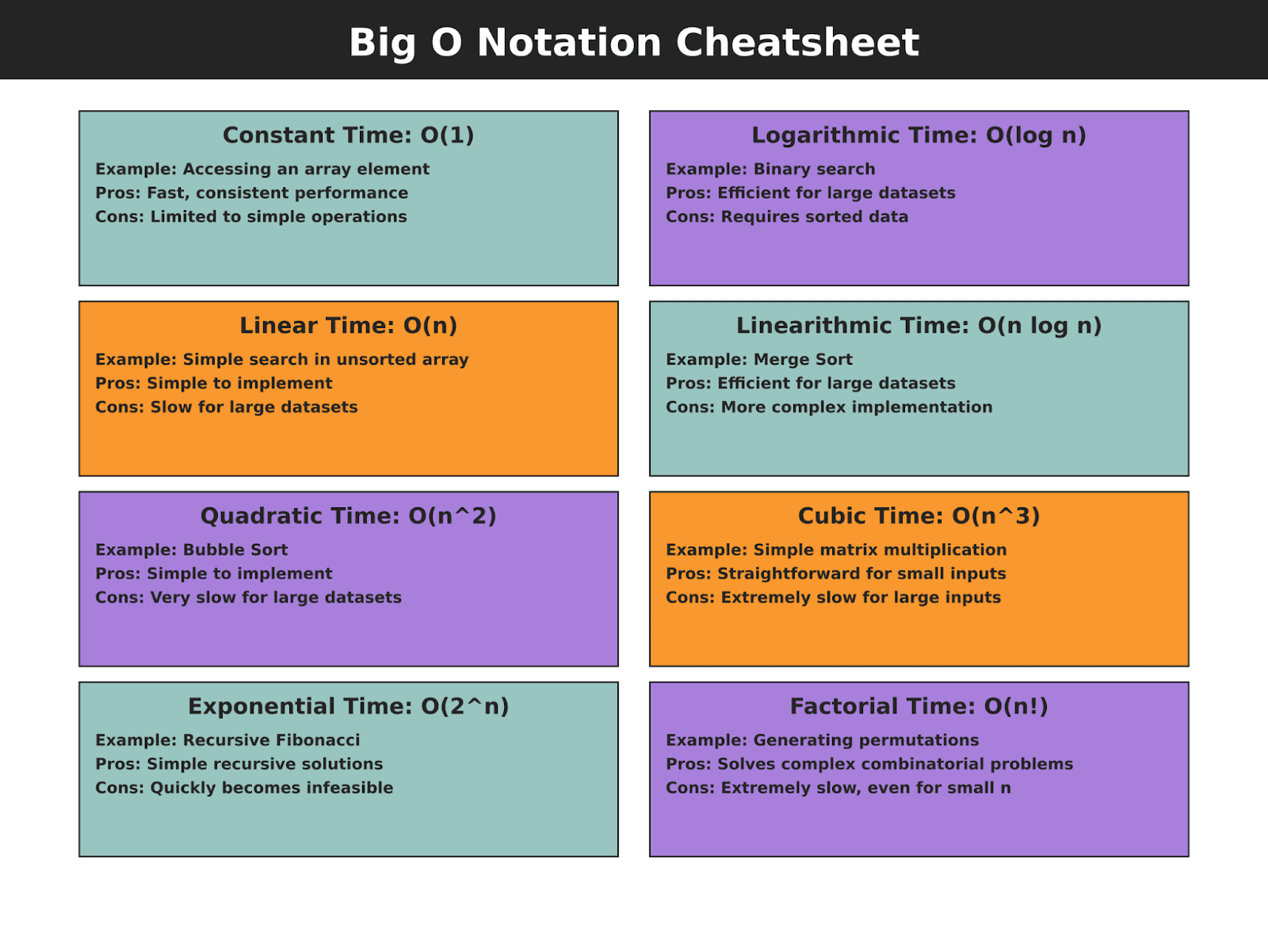
Big O Notation Cheat Sheet

Conclusion

In this article, we have explored different types of Big O Notation algorithms with many different examples.

Practice will enhance your skills! To do that, visit our platform and check our algorithm questions here. By cracking those questions, you will not only increase your algorithm skills, but you will also prepare yourself for interviews!