Top 10 Machine Learning Algorithms for Beginner Data Scientists

Let’s explore the machine learning algorithms perfect for beginners in data science. We'll explain each one and show you how to use them effectively.

Machine Learning has become an important tool in the data scientist toolkit and has become a famous concept, after seeing fancy applications in the last decade.

To effectively harness the power of machine learning, it's crucial to understand both the underlying concepts and their practical applications.

In this article, we will explore the top 10 machine learning algorithms that are particularly well-suited for those starting their journey in data science, and how to apply them. Let’s start!

1. Linear Regression

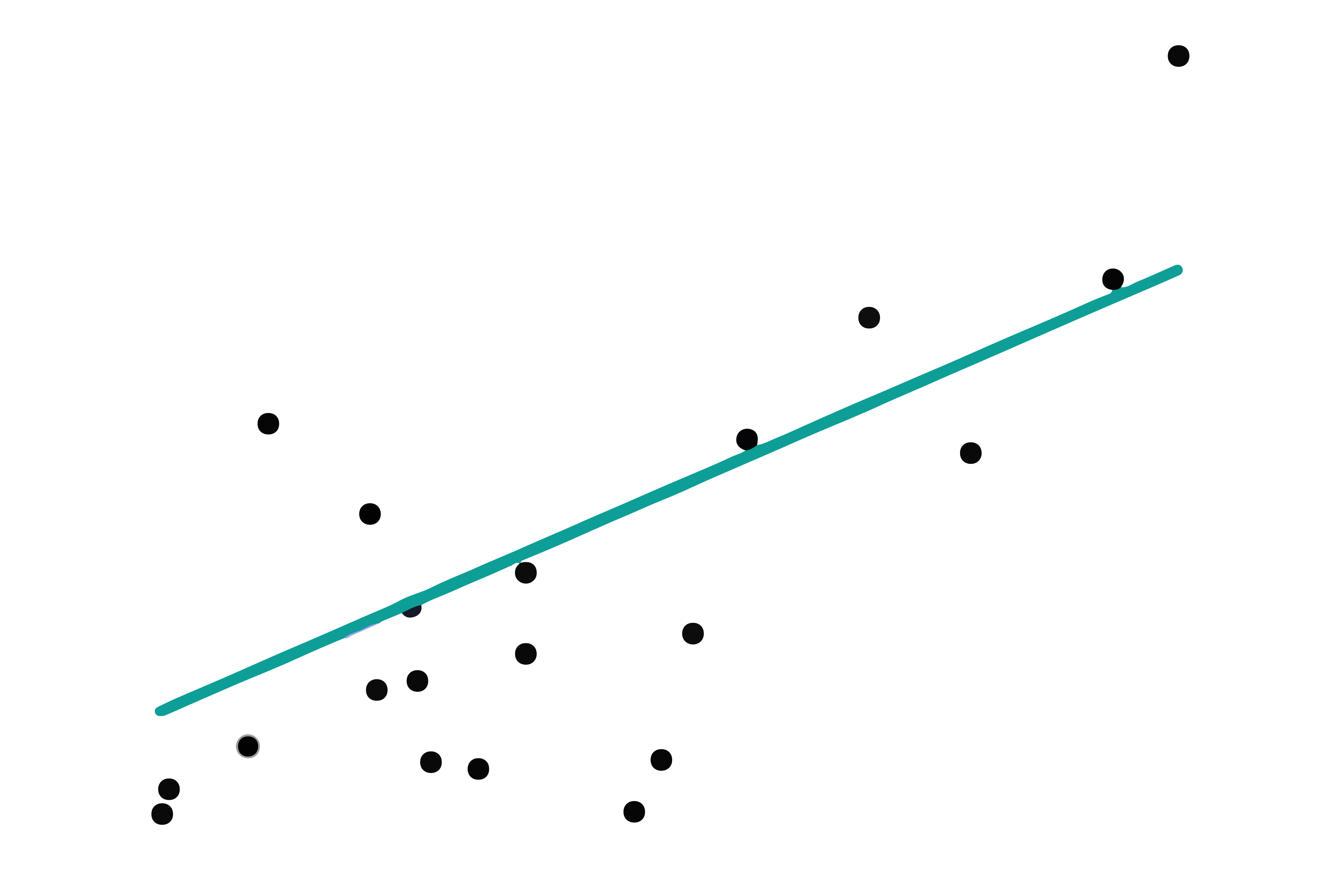
Linear Regression predicts a continuous output by establishing a linear relationship between input variables and the output. Imagine drawing a straight line through a set of points on a graph.

It decides by finding the line that best fits the data points. This line is determined by minimizing the difference (error) between the actual values and the predicted values from the line.

Evaluation Metrics

Mean Squared Error (MSE): Measures the average of the squares of the errors. Lower values are better.

R-squared: Represents the percentage of the dependent variable's variation that can be predicted based on the independent variables. Closer to 1 is better.

Applying with Sci-kit Learn

Since we're discussing Linear Regression first, we'll use the Diabetes dataset, a preloaded dataset in scikit-learn, ideal for regression tasks.

Here are the steps we’ll follow in the code blocks below;

1. Get the Diabetes Dataset loaded: Ten baseline variables, including age, sex, BMI, average blood pressure, and six blood serum measures for diabetic patients, are included in this dataset.
2. Split the Dataset: Divide it into training and testing sets.
3. Create and Train the Linear Regression Model: Build the model using the training set.
4. Predict and Evaluate: Use the test set to make predictions and then evaluate the model using MSE and R-squared.

Now let’s start!

from sklearn.datasets import load_diabetes
from sklearn.model_selection import train_test_split
from sklearn.linear_model import LinearRegression
from sklearn.metrics import mean_squared_error, r2_score

# Load the Diabetes dataset
diabetes = load_diabetes()
X, y = diabetes.data, diabetes.target

# Splitting the dataset into training and testing sets
X_train, X_test, y_train, y_test = train_test_split(X, y, test_size=0.2, random_state=42)

# Creating and training the Linear Regression model
model = LinearRegression()
model.fit(X_train, y_train)

# Predicting the test set results
y_pred = model.predict(X_test)

# Evaluating the model
mse = mean_squared_error(y_test, y_pred)
r2 = r2_score(y_test, y_pred)

print("MSE is:", mse)
print("R2 score is:", r2)

Here is the output.

These results indicate that our Linear Regression model explains about 45% of the variance in the diabetes dataset. The MSE tells us that, on average, our predictions are about 2900 units away from the true values.

2. Logistic Regression

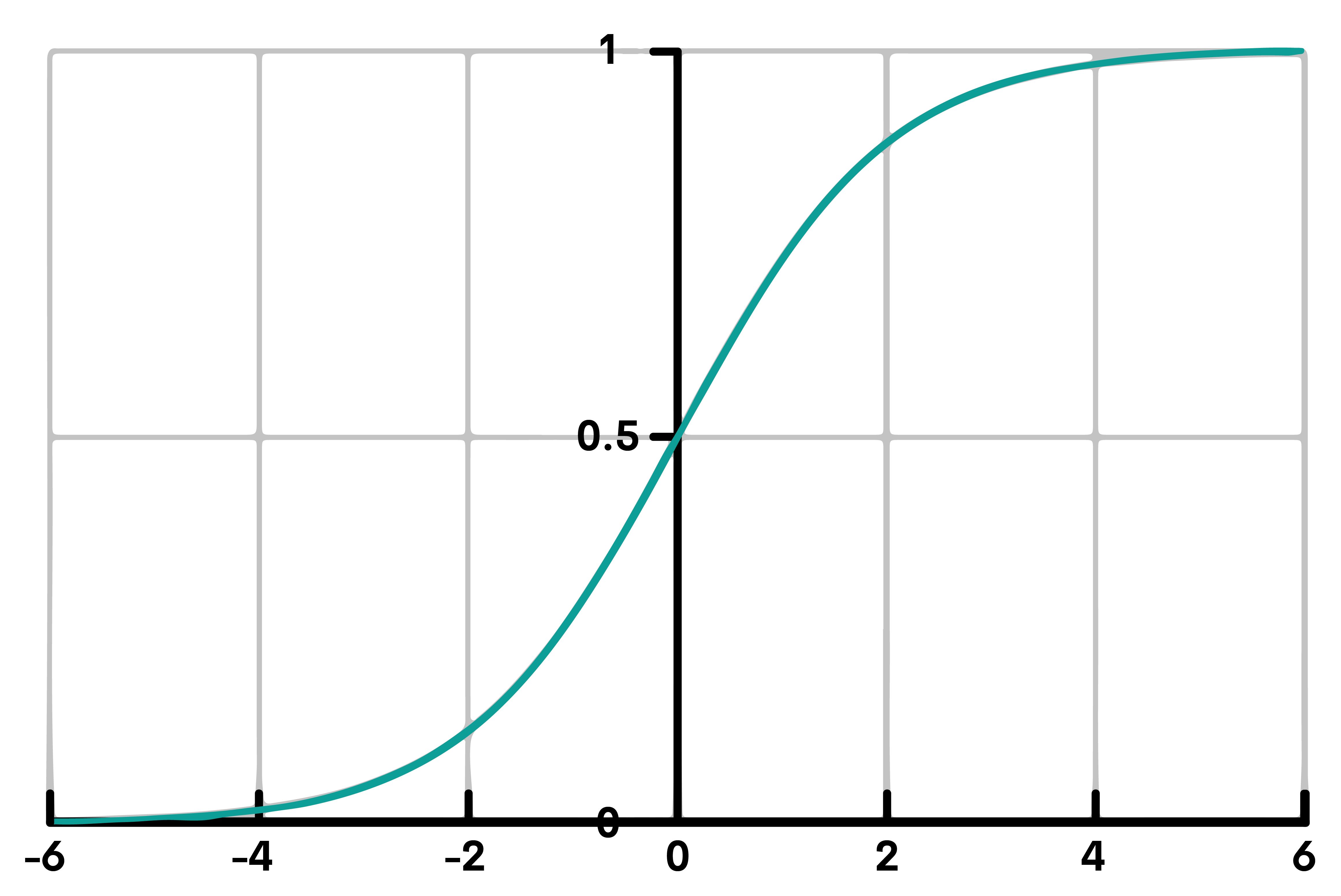
Logistic Regression is used for classification problems. It predicts the probability that a given data point belongs to a certain class, like yes/no or 0/1. It uses a logistic function to output a value between 0 and 1. This value is then mapped to a specific class based on a threshold (usually 0.5).

Evaluation Metrics

• Accuracy: Accuracy is the ratio of correctly predicted observations to total observations.
• Precision and Recall: Precision is the ratio of correctly predicted positive observations to all expected positive observations. Recall is the proportion of correctly predicted positive observations to all observations made in the actual class.
• F1 Score: An equilibrium between recall and precision.

Applying with Sci-kit Learn

Breast Cancer dataset, another preloaded dataset in scikit-learn. It's used for binary classification, making it suitable for Logistic Regression.

Here are the steps we’ll follow to apply logistic regression.

1. Load the Breast Cancer Dataset: This dataset contains features computed from a digitized image of a fine needle aspirate (FNA) of a breast mass, and the goal is to classify them as benign or malignant.
2. Split the Dataset: Divide it into training and testing sets.
3. Create and Train the Logistic Regression Model: Build the model using the training set.
4. Predict and Evaluate: Use the test set to make predictions and then evaluate the model using Accuracy, Precision, Recall, and F1 Score.
   

Let’s see the code.

from sklearn.datasets import load_breast_cancer
from sklearn.linear_model import LogisticRegression
from sklearn.model_selection import train_test_split
from sklearn.metrics import accuracy_score, precision_score, recall_score, f1_score


# Load the Breast Cancer dataset
breast_cancer = load_breast_cancer()
X, y = breast_cancer.data, breast_cancer.target

# Splitting the dataset into training and testing sets
X_train, X_test, y_train, y_test = train_test_split(X, y, test_size=0.2, random_state=42)

# Creating and training the Logistic Regression model
model = LogisticRegression(max_iter=10000)
model.fit(X_train, y_train)

# Predicting the test set results
y_pred = model.predict(X_test)

# Evaluating the model
accuracy = accuracy_score(y_test, y_pred)
precision = precision_score(y_test, y_pred)
recall = recall_score(y_test, y_pred)
f1 = f1_score(y_test, y_pred)

# Print the results
print("Accuracy:", accuracy)
print("Precision:", precision)
print("Recall:", recall)
print("F1 Score:", f1)

Here is the output.

The high recall indicates that the model is particularly good at identifying malignant cases, which is crucial in medical diagnostics.

3. Decision Trees

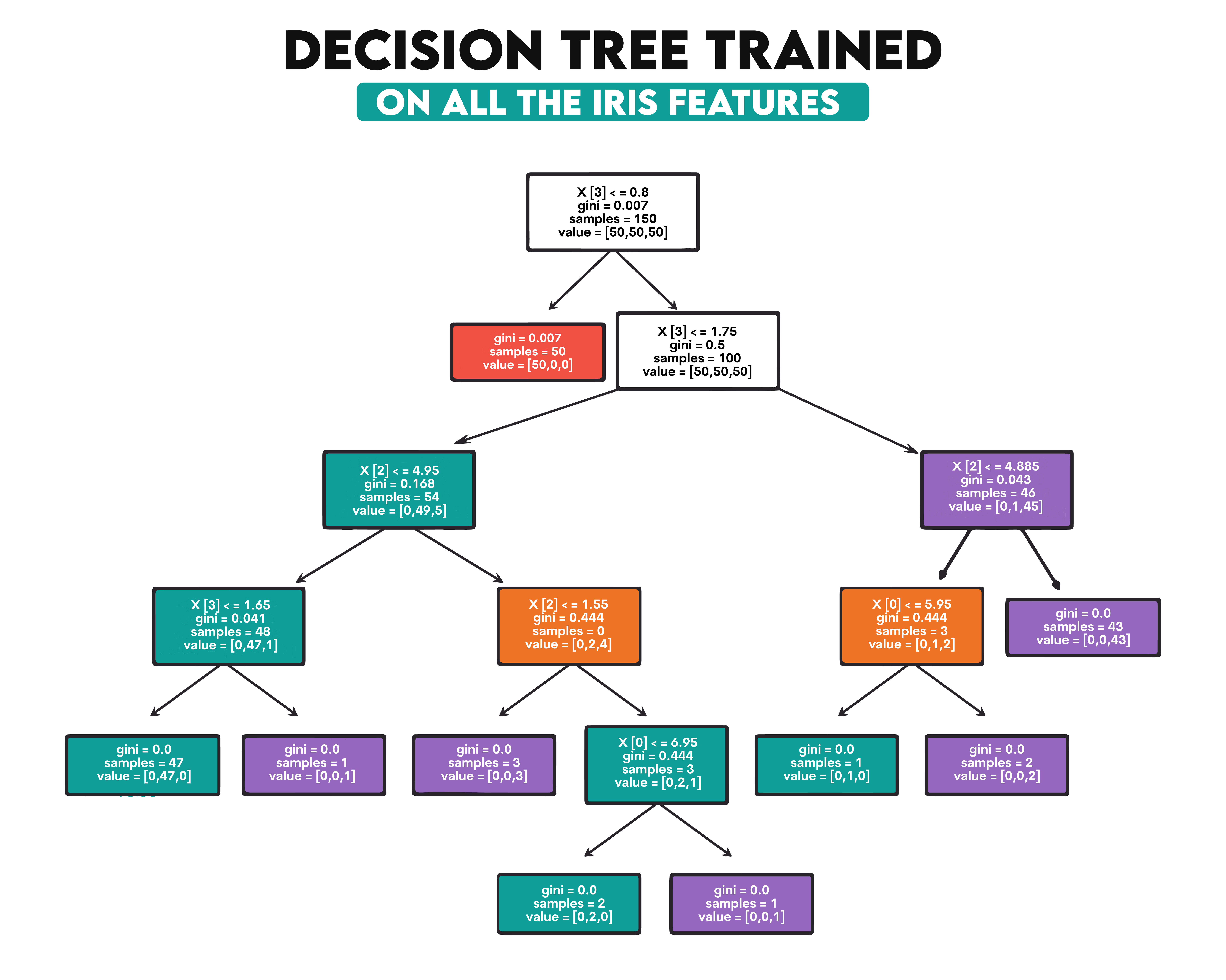
Decision Trees are like flowcharts, splitting the data based on certain conditions or features. They are applied to regression as well as classification.

The way it operates is by using feature values to split the dataset into more manageable subgroups.  Every internal node symbolizes an attribute test, every branch denotes the test's result, and every leaf node represents a class label (decision).

Evaluation Metrics

• For classification: Accuracy, precision, recall, and F1 score.
• For Regression: Mean Squared Error (MSE), R-squared.

Applying with Sci-kit Learn

We'll use the Wine dataset for Decision Trees, a classification task. This dataset is about classifying wines into three types based on different attributes. We'll train the model, predict wine types, and evaluate it using classification metrics.

Here are the steps we’ll follow in the code below.

1. Load the Wine Dataset:

• Chemical investigations of three distinct varieties of wines produced in the same region of Italy are included in the Wine dataset. Thirteen components are identified in different amounts in each of the three categories of wines by the study.

2. Split the Dataset:

• There are training and testing sets inside the dataset. This is done to train the model on one part of the data (training set) and test its performance on unseen data (testing set). We used 80% of the data for training and 20% for testing.

3. Create and Train the Decision Tree Model:

• A Decision Tree Classifier is created. This model will learn from the training data. It builds a tree-like model of decisions, where each node in the tree represents a feature of the dataset, and the branches represent decision rules, leading to different outcomes or classifications.

4. Predict and Evaluate:

• The model is used to predict the classifications of the test set. The performance of the model is then assessed by contrasting these predictions with the actual labels.

Here is the code.

from sklearn.datasets import load_wine
from sklearn.tree import DecisionTreeClassifier

# Load the Wine dataset
wine = load_wine()
X, y = wine.data, wine.target

# Splitting the dataset into training and testing sets
X_train, X_test, y_train, y_test = train_test_split(X, y, test_size=0.2, random_state=42)

# Creating and training the Decision Tree model
model = DecisionTreeClassifier(random_state=42)
model.fit(X_train, y_train)

# Predicting the test set results
y_pred = model.predict(X_test)

# Evaluating the model
accuracy = accuracy_score(y_test, y_pred)
precision = precision_score(y_test, y_pred, average='macro')
recall = recall_score(y_test, y_pred, average='macro')
f1 = f1_score(y_test, y_pred, average='macro')

# Print the results
print("Accuracy:", accuracy)
print("Precision:", precision)
print("Recall:", recall)
print("F1 Score:", f1)

Here is the output.

These results indicate that the Decision Tree model performs very well on this dataset. The high precision suggests that when it predicts a particular class of wine, it's usually correct.

4. Naive Bayes

"Naive Bayes classifiers" are a family of simple "probabilistic classifiers" that use the Bayes theorem and strong (naive) independence assumptions between the features. It’s particularly used in text classification.

It calculates the probability of each class and the conditional probability of each class given each input value. These probabilities are then used to classify a new value based on the highest probability.

Evaluation Metrics:

• Accuracy: Measures overall correctness of the model.
• Precision, Recall, and F1 Score: Especially important in cases where class distribution is imbalanced.

Applying with Sci-kit Learn

We'll use the Digits dataset, which involves classifying images of handwritten digits (0-9). This is a multi-class classification problem. We'll train the Naive Bayes model, predict digit classes, and evaluate using classification metrics. Here are the steps we’ll follow.

1. Load the Digits Dataset:

• The Digits dataset consists of 8x8 pixel images of handwritten digits (from 0 to 9). Each image is represented as a feature vector of 64 values (8x8 pixels), each representing the grayscale intensity of a pixel.

2. Split the Dataset:

• Similar to previous examples, the dataset is divided into training and testing sets. We use 80% of the data for training and 20% for testing. This helps in training the model on a large portion of the data and then evaluating its performance on a separate set that it hasn't seen before.

3. Create and Train the Naive Bayes Model:

• A Gaussian Naive Bayes classifier is created. This variant of Naive Bayes assumes that the continuous values associated with each feature are distributed according to a Gaussian (normal) distribution.
• The model is then trained (fitted) on the training data. It learns to associate the input features (pixel values) with the target values (digit classes).

4. Predict and Evaluate:

• After training, the model is used to predict the class labels of the test data.

Here is the code below.

from sklearn.datasets import load_digits
from sklearn.naive_bayes import GaussianNB

# Load the Digits dataset
digits = load_digits()
X, y = digits.data, digits.target

# Splitting the dataset into training and testing sets
X_train, X_test, y_train, y_test = train_test_split(X, y, test_size=0.2, random_state=42)

# Creating and training the Naive Bayes model
model = GaussianNB()
model.fit(X_train, y_train)

# Predicting the test set results
y_pred = model.predict(X_test)

# Evaluating the model
accuracy = accuracy_score(y_test, y_pred)
precision = precision_score(y_test, y_pred, average='macro')
recall = recall_score(y_test, y_pred, average='macro')
f1 = f1_score(y_test, y_pred, average='macro')

# Print the results
print("Accuracy:", accuracy)
print("Precision:", precision)
print("Recall:", recall)
print("F1 Score:", f1)

Here is the output.

These results show that the Naive Bayes model has a good performance on this dataset, with fairly balanced precision and recall. The model is quite effective in classifying handwritten digits, though there's room for improvement, especially in terms of accuracy and F1 score.

5. K-Nearest Neighbors (KNN)

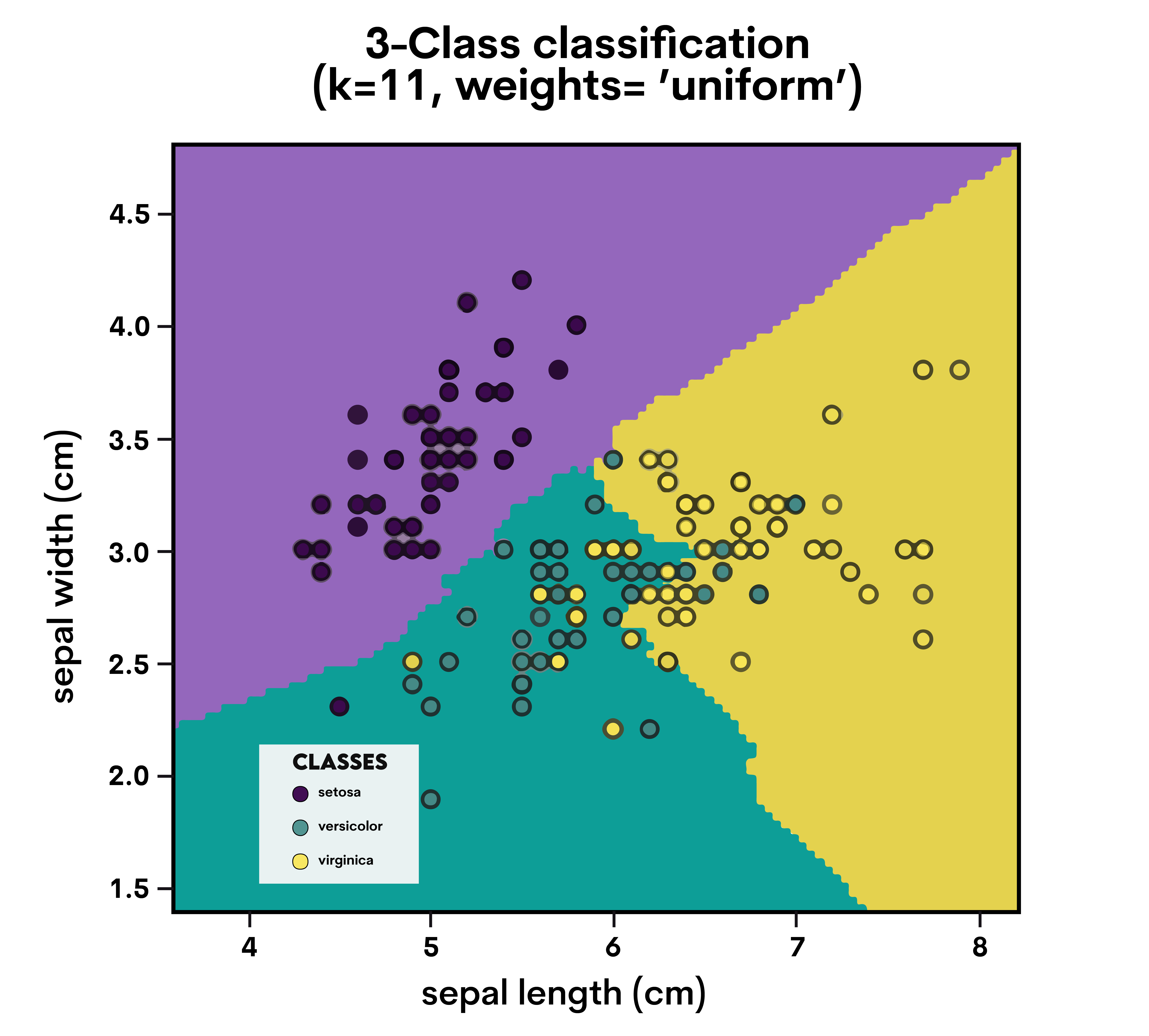
An easy-to-understand approach for regression and classification is K-Nearest Neighbors (KNN). A data point is classed according to the classification of its neighbors.

KNN looks at the 'K' closest points (neighbors) to a data point and classifies it based on the majority class of these neighbors. For regression, it takes the average of the 'K' nearest points.

Evaluation Metrics

• Classification: Accuracy, Precision, Recall, F1 Score.
• Regression: Mean Squared Error (MSE), R-squared.

Applying with Sci-kit Learn

We'll use the Wine dataset again but this time with KNN. We'll train the KNN model to classify the types of wine and evaluate its performance with classification metrics. Here are the steps we’ll follow.

1. Create and Train the KNN Model:

• A K-Nearest Neighbors (KNN) model is created with n_neighbors=3. This means the model looks at the three nearest neighbors of a data point to make a prediction.
• The model is trained (fitted) with the training data. During training, it doesn't build a traditional model but memorizes the dataset.

2. Predict:

• The trained KNN model is then used to predict the class labels (types of wine) of the test data. The model determines the most common class among these neighbors for each point in the test set by examining the three nearest points in the training set

3. Evaluate:

• The model's predictions are evaluated against the actual labels of the test set.

Here is the code.

from sklearn.datasets import load_wine
from sklearn.model_selection import train_test_split
from sklearn.neighbors import KNeighborsClassifier
from sklearn.metrics import accuracy_score, precision_score, recall_score, f1_score

# Load the Wine dataset
wine = load_wine()
X, y = wine.data, wine.target

# Splitting the dataset into training and testing sets
X_train, X_test, y_train, y_test = train_test_split(X, y, test_size=0.2, random_state=42)

# Creating and training the KNN model
knn_model = KNeighborsClassifier(n_neighbors=3)
knn_model.fit(X_train, y_train)

# Predicting the test set results
y_pred_knn = knn_model.predict(X_test)

# Evaluating the model
accuracy_knn = accuracy_score(y_test, y_pred_knn)
precision_knn = precision_score(y_test, y_pred_knn, average='macro')
recall_knn = recall_score(y_test, y_pred_knn, average='macro')
f1_knn = f1_score(y_test, y_pred_knn, average='macro')

# Print the results
print("Accuracy:", accuracy_knn)
print("Precision:", precision_knn)
print("Recall:", recall_knn)
print("F1 Score:", f1_knn)

Here is the output.

These results indicate that the KNN model performs exceptionally well on this dataset. The high scores across all metrics show that the model is not only accurate overall but also maintains a good balance between precision and recall, effectively classifying the wine types.

6. Support Vector Machines (SVM)

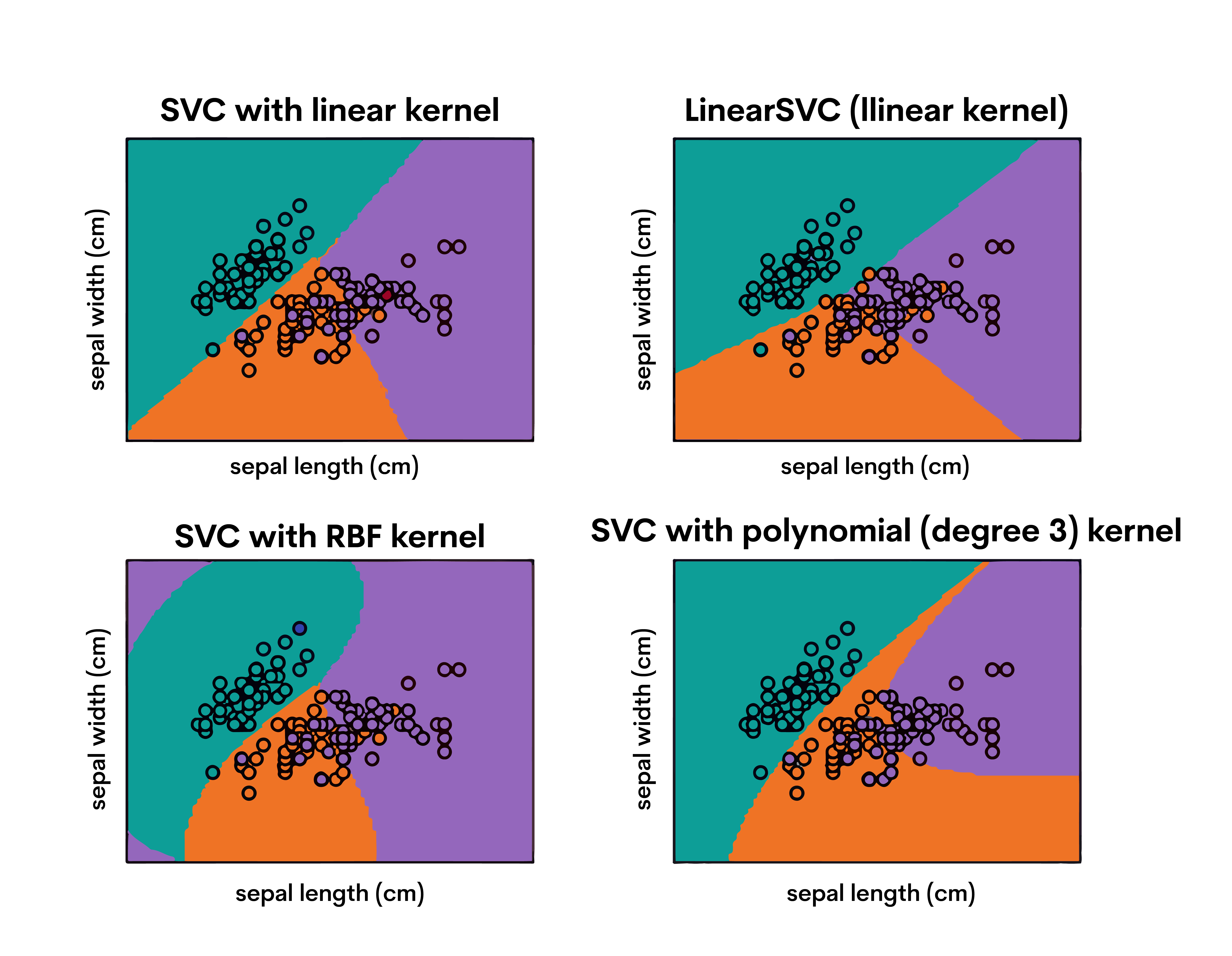
Support Vector Machines (SVM) are powerful and versatile supervised learning models, used for both classification and regression tasks. They work well for complex datasets.

SVM constructs a hyperplane (or set of hyperplanes) in a high-dimensional space to separate different classes. It aims to find the best margin (distance between the line and the nearest points of each class, known as support vectors) that separates the classes.

Evaluation Metrics

• Classification: Accuracy, Precision, Recall, F1 Score.
• Regression: Mean Squared Error (MSE), R-squared.

Applying with Sci-kit Learn

We'll apply SVM to the Breast Cancer dataset, focusing on classifying tumors as benign or malignant. We'll train the SVM model and evaluate its performance using classification metrics.

Here are the steps we’ll follow;

1. Create and Train the SVM Model:

• A Support Vector Machine (SVM) model is created using the default settings. SVM is known for its ability to create a hyperplane (or multiple hyperplanes in higher-dimensional spaces) that separates the classes with as wide a margin as possible.

2. Predict:

• The trained SVM model is then used to predict the class labels of the test data. It does this by determining on which side of the hyperplane each data point falls.

3. Evaluate:

• The model's predictions are evaluated against the actual labels of the test set to assess its performance.

Here is the code.

from sklearn.svm import SVC

breast_cancer = load_breast_cancer()
X, y = breast_cancer.data, breast_cancer.target

# Splitting the dataset into training and testing sets
X_train, X_test, y_train, y_test = train_test_split(X, y, test_size=0.2, random_state=42)

# Creating and training the SVM model
svm_model = SVC()
svm_model.fit(X_train, y_train)

# Predicting the test set results
y_pred_svm = svm_model.predict(X_test)

# Evaluating the model
accuracy_svm = accuracy_score(y_test, y_pred_svm)
precision_svm = precision_score(y_test, y_pred_svm, average='macro')
recall_svm = recall_score(y_test, y_pred_svm, average='macro')
f1_svm = f1_score(y_test, y_pred_svm, average='macro')

accuracy_svm, precision_svm, recall_svm, f1_svm

# Print the results
print("Accuracy:", accuracy_svm)
print("Precision:", precision_svm)
print("Recall:", recall_svm)
print("F1 Score:", f1_svm)

Here is the output.

These results indicate that the SVM model performs exceptionally well on the Breast Cancer dataset. The high accuracy, precision, recall, and F1 scores demonstrate the model's effectiveness in distinguishing between benign and malignant tumors.

The balance between precision and recall is particularly important in medical diagnoses, where both false positives and false negatives carry significant consequences.

7. Random Forest

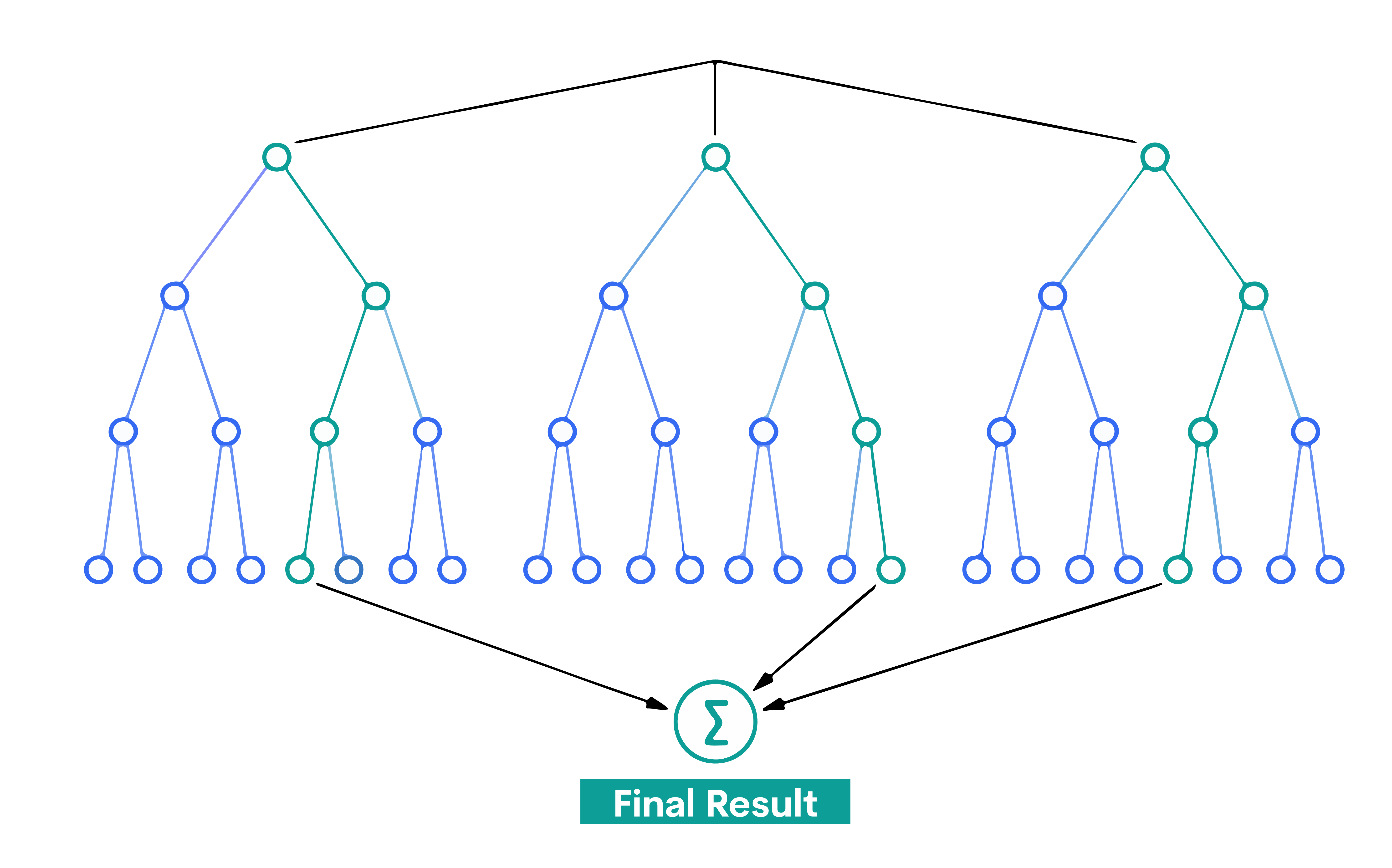
One ensemble learning technique that's typically utilized for regression and classification is called Random Forest. To provide a forecast that is more reliable and accurate, it constructs many decision trees and blends them.

Every tree in a Random Forest makes a forecast, and the model's prediction (for classification) belongs to the class that receives the most votes. For regression, it takes the average of outputs by different trees.

Evaluation Metrics:

• Classification: Accuracy, Precision, Recall, F1 Score.
• Regression: Mean Squared Error (MSE), R-squared.

Applying with Sci-kit Learn

We'll apply Random Forest to the Breast Cancer dataset for classifying tumors as benign or malignant. We'll train the Random Forest model and evaluate its performance using classification metrics.

1. Create and Train the Random Forest Model:

• Initialize a Random Forest Classifier.
• Utilizing the training data, fit (train) the model.

2. Predict:

• Use the trained model to predict the labels of the test data.

3. Evaluate:

• Assess the model's performance on the test data using Accuracy, Precision, Recall, and F1 Score.

Let’s see the code.

from sklearn.ensemble import RandomForestClassifier

breast_cancer = load_breast_cancer()
X, y = breast_cancer.data, breast_cancer.target

# Splitting the dataset into training and testing sets
X_train, X_test, y_train, y_test = train_test_split(X, y, test_size=0.2, random_state=42)


# Creating and training the Random Forest model
rf_model = RandomForestClassifier(random_state=42)
rf_model.fit(X_train, y_train)

# Predicting the test set results
y_pred_rf = rf_model.predict(X_test)

# Evaluating the model
accuracy_rf = accuracy_score(y_test, y_pred_rf)
precision_rf = precision_score(y_test, y_pred_rf, average='macro')
recall_rf = recall_score(y_test, y_pred_rf, average='macro')
f1_rf = f1_score(y_test, y_pred_rf, average='macro')

# Print the results
print("Accuracy:", accuracy)
print("Precision:", precision)
print("Recall:", recall)
print("F1 Score:", f1)

Here is the output.

These results demonstrate that the Random Forest model has a high level of performance on the Breast Cancer dataset, with strong scores across all key metrics.

The high precision and recall suggest that the model is effective in accurately identifying both benign and malignant tumors, with a balanced approach to minimizing both false positives and false negatives.

8. K-Means Clustering

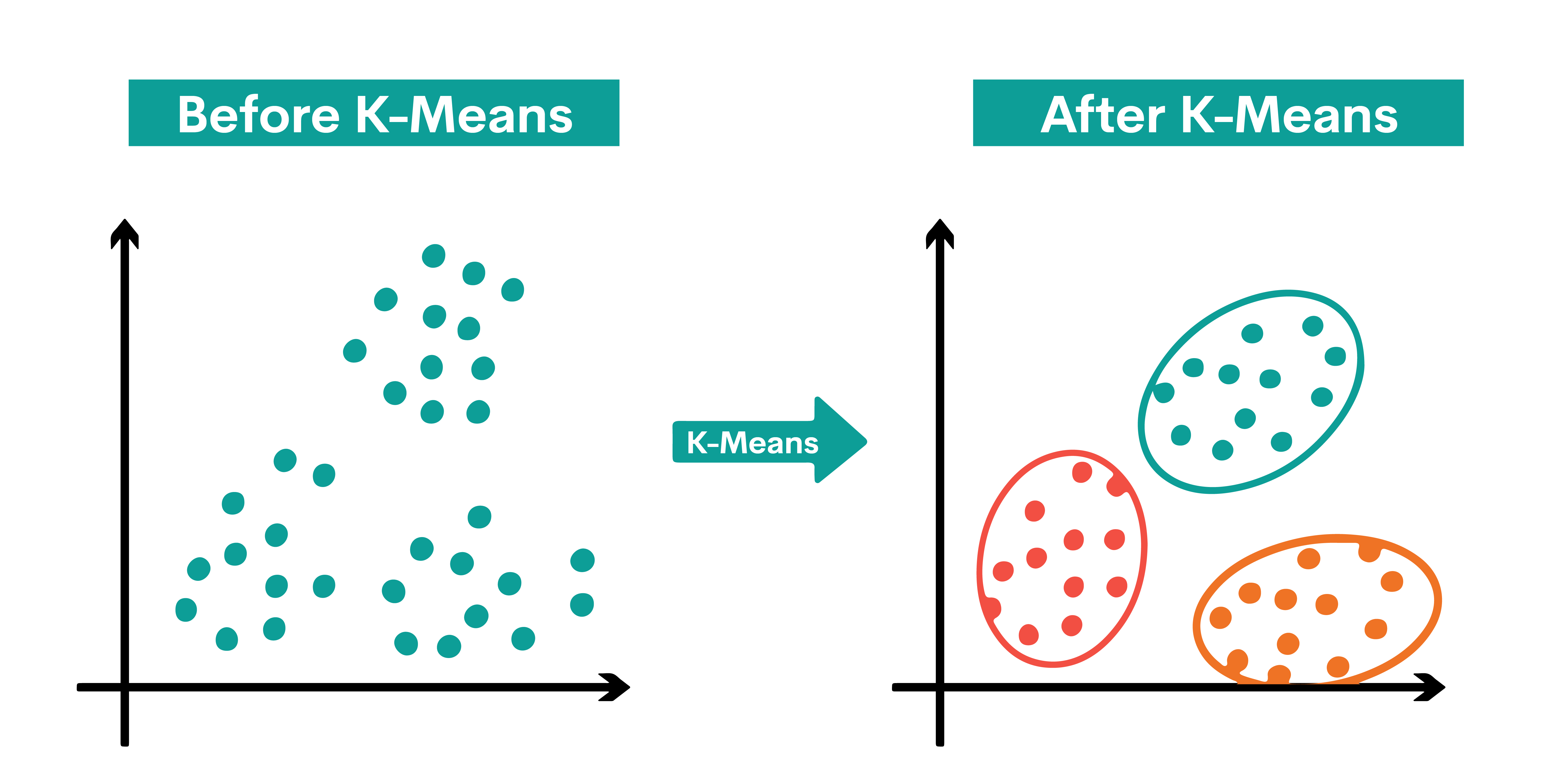
K-Means Clustering is an unsupervised learning algorithm used for grouping data into 'K' clusters. After identifying k centroids, each data point is assigned to the closest cluster with the goal of minimizing the size of the centroids.

The algorithm assigns data points to a cluster such that the sum of the squared distance between the data points and the cluster's centroid is at the minimum. The homogeneity of data points inside a cluster increases with decreasing variance within the cluster.

Evaluation Metrics

• Inertia: The total squared distance of the samples to the nearest cluster center is known as inertia. It is better to have lower values.
• Silhouette Score: Indicates how cohesively an item belongs to its own cluster as opposed to how much it separates from other clusters. A high silhouette score means that the item is well matched to its own cluster and poorly matched to nearby clusters. The silhouette score goes from -1 to 1.

Applying with Sci-kit Learn

Let’s use the Iris dataset for K-Means Clustering. The task will be to group the iris plants into clusters based on their flower measurements. We'll train the model, assign the plants to clusters, and evaluate the clustering.

1. Load the Iris Dataset:

• The Iris dataset contains measurements of iris flowers, including sepal length, sepal width, petal length, and petal width. The dataset is typically used for classification tasks, but here we'll use it for clustering.

2. Apply K-Means Clustering:

• We initialize a K-Means clustering algorithm with n_clusters=3, as there are three species of iris in the dataset. However, the algorithm is unaware of these species; it will simply try to find the best way to group the data into three clusters.
• We fit the model to the data X, which includes our four features. The K-Means algorithm iteratively assigns each data point to one of the three clusters based on the distance of the data point to the cluster centroids.

3. Predict Clusters:

• The predict method is used to assign each data point in X to one of the three clusters. This step is somewhat conceptual with K-Means since the fitting and prediction happen together, but essentially, each data point is now labeled with a cluster number.

4. Evaluate the Clustering:

• We evaluate our clustering using two metrics:
  • Inertia: This is the sum of squared distances of samples to their closest cluster center. It’s a measure of how internally coherent clusters are. We aim for lower inertia.
  • Silhouette Score: This measures how similar an object is to its own cluster (cohesion) compared to other clusters (separation). The silhouette score ranges from -1 to 1, where a high value indicates that the object is well matched to its own cluster and poorly matched to neighboring clusters.

Let’s see the code.

from sklearn.datasets import load_iris
from sklearn.cluster import KMeans
from sklearn.metrics import silhouette_score

# Load the Iris dataset
iris = load_iris()
X = iris.data

# Applying K-Means Clustering
kmeans = KMeans(n_clusters=3, random_state=42)
kmeans.fit(X)

# Predicting the cluster for each data point
y_pred_clusters = kmeans.predict(X)

# Evaluating the model
inertia = kmeans.inertia_
silhouette = silhouette_score(X, y_pred_clusters)

print("Inertia:", inertia)
print("Silhouette:", silhouette)

Here is the output.

These metrics suggest that the K-Means algorithm has performed reasonably well in clustering the Iris dataset, though there's room for improvement in terms of cluster compactness and separation.

9. Principal Component Analysis (PCA)

Dimensionality reduction is accomplished by the use of Principal Component Analysis (PCA). It transforms the data into a new coordinate system, reducing the number of variables while preserving as much of the original data's variation as possible.

The primary components, or axis, that maximize the variance in the data are found using PCA. The first principal component captures the most variance, the second principal component (orthogonal to the first) captures the next most, and so on.

Evaluation Metrics

• Explained Variance: Indicates how much variance in the data is captured by each principal component.
• Total Explained Variance: The cumulative variance explained by the selected principal components.

Applying with Sci-kit Learn

The Breast Cancer dataset, which includes characteristics derived from a digital picture of a fine needle aspirate (FNA) of a breast tumor, will be subjected to PCA. Our objective is to minimize the dataset's dimensionality while maintaining the greatest amount of information.

Here are the steps we’ll follow:

1. Load the Breast Cancer Dataset:

• The Breast Cancer dataset consists of features computed from digitized images of fine needle aspirates of breast masses. The features are attributes of the cell nuclei that are visible in the picture.

2. Apply PCA:

• We initialize PCA with n_components=2, indicating our intention to reduce the dataset to two dimensions. This choice is often made for visualization purposes or as a pre-processing step for other algorithms.
• We fit PCA to the data X. During this process, PCA identifies the axes (principal components) that account for the most variance in the data.

3. Transform the Data:

• The transform method of PCA is used to apply the dimensionality reduction to X. This results in a new dataset X_pca, where each data point is now represented in terms of the two principal components.

4. Evaluate the PCA Transformation:

• We evaluate our PCA transformation by looking at the Explained Variance of each principal component. This tells us how much of the data's total variance is captured by each principal component.
• The Total Explained Variance is calculated by summing the explained variances of the two principal components. This gives us an overall measure of how much information was preserved in the dimensionality reduction process.

Now let’s see the code.

from sklearn.datasets import load_breast_cancer
from sklearn.decomposition import PCA
import numpy as np

# Load the Breast Cancer dataset
breast_cancer = load_breast_cancer()
X = breast_cancer.data

# Applying PCA
pca = PCA(n_components=2)  # Reducing to 2 dimensions for simplicity
pca.fit(X)

# Transforming the data
X_pca = pca.transform(X)

# Explained Variance
explained_variance = pca.explained_variance_ratio_

# Total Explained Variance
total_explained_variance = np.sum(explained_variance)

print("Explained variance:", explained_variance)
print("Total Explained Variance:", total_explained_variance)

Let’s see the result.

Let’s evaluate the results.

Explained Variance:

• First Principal Component: 98.20%
• Second Principal Component: 1.62%
• Total Explained Variance: 99.82%

These results indicate that by reducing the dataset to just two principal components, we have captured approximately 99.82% of the total variance in the dataset.

The first component alone accounts for a significant majority of this variance, which suggests that it captures most of the essential information present in the dataset.

10. Gradient Boosting Algorithms

Gradient Boosting is an advanced machine learning technique. It builds multiple weak predictive models (usually decision trees) sequentially. Each new model gradually minimizes the loss function (error) of the whole system.

Three components are involved: an additive model that adds weak learners to minimize the loss function, a loss function that has to be optimized, and a weak learner that needs to generate predictions. Every new tree fixes the mistakes made by the ones before it.

Evaluation Metrics

• For Classification: Accuracy, Precision, Recall, F1 Score.
• For Regression: Mean Squared Error (MSE), R-squared.

Applying with Sci-kit Learn

We'll use the Diabetes dataset for Gradient Boosting. Our goal will be to predict the progression of diabetes based on various features. We'll train a gradient-boosting model and evaluate its performance.

Let’s see the steps we’ll follow below:

1. Load the Diabetes Dataset

• Age, sex, body mass index, average blood pressure, and six blood serum measures are among the characteristics that are included in the Diabetes dataset. One year after baseline, a quantitative assessment of the disease's development is the goal variable.

2. Create and Train the Gradient Boosting Model:

• We initialize a Gradient Boosting Regressor. Gradient Boosting permits the optimization of any differentiable loss function and constructs an additive model in a forward, step-by-step manner
• We train (fit) this model on the training data. In this step, the model learns to predict the diabetes progression based on the features.

3. Predict:

• We use the trained Gradient Boosting model to predict the disease progression on the test data. This step involves applying the model to unseen data to assess its predictive capabilities.

4. Evaluate:

• The model's performance is assessed using two key metrics:
  • Mean Squared Error (MSE): The average of the squares of the mistakes is what this metric calculates. It is a metric for evaluating the quality of an estimator; values nearer zero indicate greater quality.
  • R-squared: Based on the percentage of total result variance that the model explains, this statistic gives an indication of how well the observed outcomes are duplicated by the model.
    

Here is the code.

from sklearn.datasets import load_diabetes
from sklearn.ensemble import GradientBoostingRegressor
from sklearn.metrics import mean_squared_error, r2_score

# Load the Diabetes dataset
diabetes = load_diabetes()
X, y = diabetes.data, diabetes.target

# Splitting the dataset into training and testing sets
X_train, X_test, y_train, y_test = train_test_split(X, y, test_size=0.2, random_state=42)

# Creating and training the Gradient Boosting model
gb_model = GradientBoostingRegressor(random_state=42)
gb_model.fit(X_train, y_train)

# Predicting the test set results
y_pred_gb = gb_model.predict(X_test)

# Evaluating the model
mse_gb = mean_squared_error(y_test, y_pred_gb)
r2_gb = r2_score(y_test, y_pred_gb)

print("MSE:", mse_gb)
print("R2 score:", r2_gb)

Here is the output.

These results indicate that the gradient-boosting model has a moderate level of accuracy in predicting diabetes progression.

The R-squared value of 0.45 suggests that nearly 45% of the variance in the target variable is explained by the model, which is decent for a complex task like this.

The MSE gives us an idea of the average squared difference between the observed actual outcomes and the outcomes predicted by the model.

Final Thoughts

In this article, we've reviewed the top 10 machine learning algorithms essential for any budding data scientist.

Remember, consistent practice and application in real-world scenarios is the key to mastering these algorithms.

If you're interested in delving further, take a look at this article discussing Machine Learning Algorithms.

Stay motivated and join StrataScratch, where you can dive into engaging data projects and tackle data science interview questions, setting you on a successful path in your data science journey.