SQL Aggregate Functions Interview Questions

Categories:
 Written by:
Vivek Sankaran
Let's take a deeper dive into the must-know SQL aggregate concepts for your next Data Science Interview.
Today, we have millions and billions of rows of data being generated each second. However, we usually need a single metric to flag changes and make business decisions. For example - the total sales in the last quarter, the average churn rate, the number of ad impressions served, etc. Aggregation functions help generate these metrics. Aggregate functions compute a single result from a set of input values. All aggregate functions are deterministic - they output the same value every time they are invoked with the same set of input values. We have an article “The Ultimate Guide to SQL Aggregate Functions” to get an introductory overview of these functions. In this article, we take a deeper dive into using SQL aggregation functions. The various scenarios that we will discuss here are -
- Aggregation on an entire table
- Aggregation by Cohorts
- Aggregation in Window Functions
Note: Except for COUNT(*), all aggregation functions neglect the NULL values unless otherwise specified. Let us get started.
Aggregation on an entire table

The simplest use case is to find the overall aggregate metric from a dataset. Let us try this with an example from a Postmates Data Scientist Interview Question.
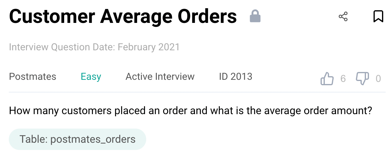
Question #1: Customer Average Orders
Find the average order amount and the number of customers who placed an order.
Link to the question: https://platform.stratascratch.com/coding/2013-customer-average-orders
This problem uses the postmates_order table with the following fields.
| id: | int |
| customer_id: | int |
| courier_id: | int |
| seller_id: | int |
| order_timestamp_utc: | datetime |
| amount: | float |
| city_id: | int |
The data is presented in the following manner.
Solution
The problem is pretty straightforward. But with a slight twist which we will come to later. Finding the average order amount is pretty easy. We simply need to use the AVG() function.
SELECT
    AVG(amount) AS avg_order_amount
FROM postmates_orders
;
However, to find the number of customers, we need to be a bit careful. We cannot simply take COUNT(*) or COUNT(customer_id) as there are customers with repeat transactions. We need to use the DISTINCT keyword to ensure that we count only uniques. The problem can be solved by using the following query.
SELECT
    COUNT(DISTINCT customer_id) AS num_customers
    , AVG(amount) AS avg_order_amount
FROM postmates_orders
;
We can also subset the dataset using the WHERE clause and then apply the aggregate over the resulting data. Let us see this in practice with a problem that came up in a Yelp Data Science Interview.
Question #2: Number of Yelp Businesses that sell Pizza
Find the number of Yelp businesses that sell pizza.

Link to the question: https://platform.stratascratch.com/coding/10153-find-the-number-of-yelp-businesses-that-sell-pizza
The problem uses the yelp_business dataset with the following fields.
| business_id: | varchar |
| name: | varchar |
| neighborhood: | varchar |
| address: | varchar |
| city: | varchar |
| state: | varchar |
| postal_code: | varchar |
| latitude: | float |
| longitude: | float |
| stars: | float |
| review_count: | int |
| is_open: | int |
| categories: | varchar |
The data looks like this.
Solution
This is a pretty easy question. There are two parts that we need to consider while solving the problem.
- Identify the businesses that sell a pizza
- Count the relevant businesses.
To identify the pizza-selling businesses, we use the categories field and search if the text contains the phrase ‘pizza’. To make the search case insensitive, we use the ILIKE operator.
SELECT business_id, categories
FROM yelp_business
WHERE categories ILIKE '%pizza%'
;
Alternatively, we can also convert the text to upper or lower case and use the LIKE operator which is available in all flavors of SQL.
SELECT business_id, categories
FROM yelp_business
WHERE LOWER(categories) LIKE '%pizza%'
;
The output looks like this
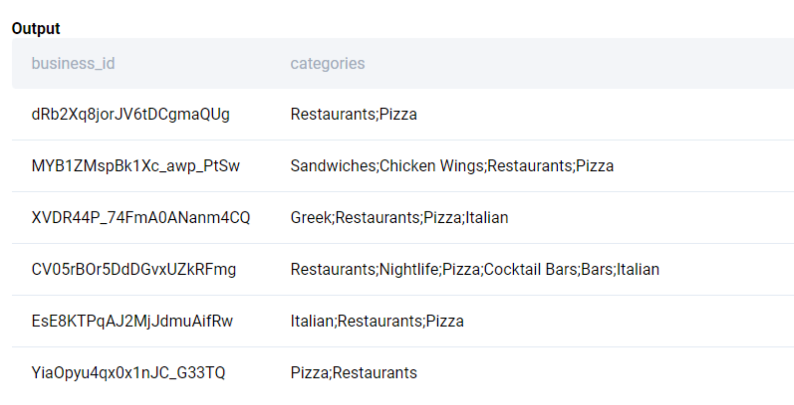
Now we simply count the unique business_id. Again, we use the DISTINCT keyword to disregard duplicates.
SELECT COUNT(DISTINCT business_id)
FROM yelp_business
WHERE LOWER(categories) LIKE '%pizza%'
;
Aggregation by cohorts

Another common use case for aggregation is to summarize by different cohorts - same product category, the month of the transaction, the week of site visit, etc. These cohort-based analyses help us identify trends in a sub-layer that might not be visible in the overall aggregates. We can accomplish this by using the GROUP BY clause. Let us start with an easy problem from an ESPN Data Science Interview.
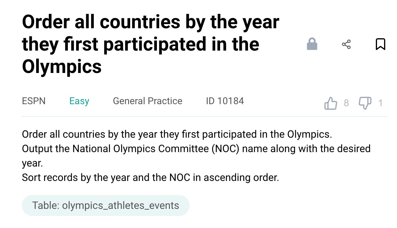
Question #3: Find the year first participated in the Olympics
Order the countries on the basis of the year they first participated in the Olympics. The country is available in the National Olympics Committee (NOC) field. Report the year and the NOC in ascending order.
Link to the question: https://platform.stratascratch.com/coding/10184-order-all-countries-by-the-year-they-first-participated-in-the-olympics
The problem uses the olympics_athletes_events dataset with the following fields.
| id: | int |
| name: | varchar |
| sex: | varchar |
| age: | float |
| height: | float |
| weight: | datetime |
| team: | varchar |
| noc: | varchar |
| games: | varchar |
| year: | int |
| season: | varchar |
| city: | varchar |
| sport: | varchar |
| event: | varchar |
| medal: | varchar |
| non_team: | datetime |
The data is presented in the following manner.
Solution
This is a relatively easy problem. To solve this we proceed in the following manner.
- Find the earliest year that a particular country participated in the Olympics.
- Order the results in the required manner.
Unlike the previous problem, we need to aggregate by the country. To do this, we use the GROUP BY clause.
SELECT
noc, MIN(year)
FROM olympics_athletes_events
GROUP BY 1
;
We get the following output.
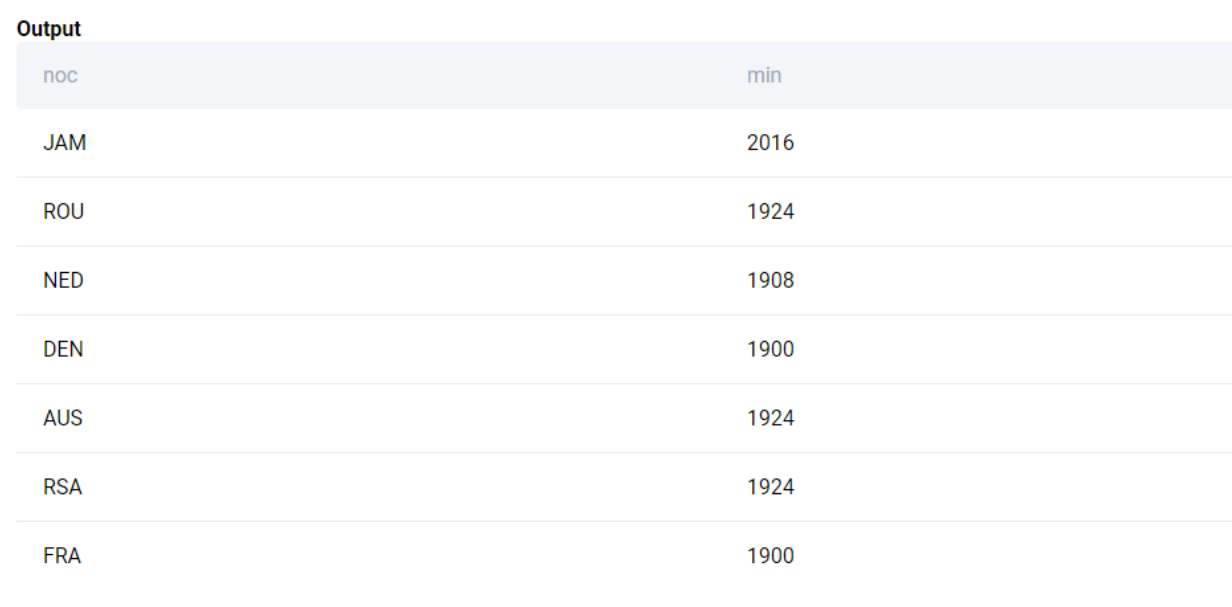
We complete the problem by ordering the output as required.
SELECT
noc, MIN(year)
FROM olympics_athletes_events
GROUP BY 1
ORDER BY 2,1
;
Let us try a slightly trickier SQL aggregate functions interview question. This one came from a City of San Francisco Data Science Interview.
Question #4: Highest Salary each year
Report the highest payment for each employee for each of the years 2011 to 2014. Output as one row per employee with the corresponding highest payments for each of the aforementioned years. Order the records in the alphabetical order of the employee's name.
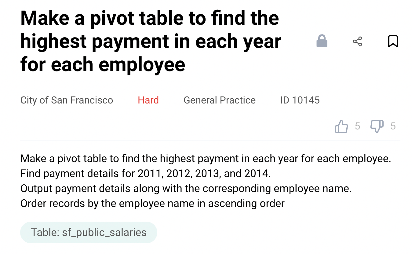
Link to the question: https://platform.stratascratch.com/coding/10145-make-a-pivot-table-to-find-the-highest-payment-in-each-year-for-each-employee
The problem uses the sf_public_salaries table with the following fields.
| id: | int |
| employeename: | varchar |
| jobtitle: | varchar |
| basepay: | float |
| overtimepay: | float |
| otherpay: | float |
| benefits: | float |
| totalpay: | float |
| totalpaybenefits: | float |
| year: | int |
| notes: | datetime |
| agency: | varchar |
| status: | varchar |
The data is presented in the following manner.
Solution
We can solve this SQL aggregate functions interview question in the following manner.
- Start by pivoting the pay for each year for each employee.
- Aggregate the data for each employee for each of the years and output in the required manner.
The columns of interest in the dataset are employeename, totalpay, and year. The data is in a long format. We need to convert it into a wide format. To do this we use the CASE WHEN operator.
SELECT
    employeename
    , CASE WHEN year = 2011 THEN totalpay ELSE 0 END AS pay_2011
    , CASE WHEN year = 2012 THEN totalpay ELSE 0 END AS pay_2012
    , CASE WHEN year = 2013 THEN totalpay ELSE 0 END AS pay_2013
    , CASE WHEN year = 2014 THEN totalpay ELSE 0 END AS pay_2014
FROM
sf_public_salaries
;
We get the following output.
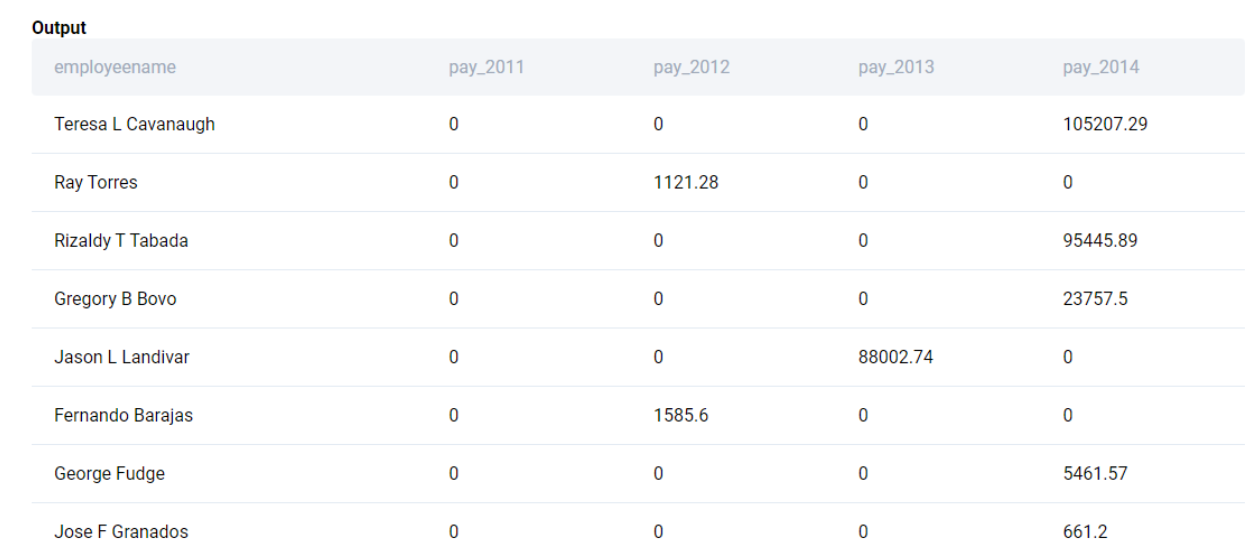
We have successfully pivoted from a long-format dataset to a wide-format dataset. Now we simply find the maximum salaries for each of the columns aggregating on the employee name and ordering the results in alphabetical order.
WITH yearly_pays as (
SELECT
    employeename
    , CASE WHEN year = 2011 THEN totalpay ELSE 0 END AS pay_2011
    , CASE WHEN year = 2012 THEN totalpay ELSE 0 END AS pay_2012
    , CASE WHEN year = 2013 THEN totalpay ELSE 0 END AS pay_2013
    , CASE WHEN year = 2014 THEN totalpay ELSE 0 END AS pay_2014
FROM
sf_public_salaries
)
SELECT
    employeename
    , MAX(pay_2011) AS pay_2011
    , MAX(pay_2012) AS pay_2012
    , MAX(pay_2013) AS pay_2013
    , MAX(pay_2014) AS pay_2014
FROM yearly_pays
GROUP BY 1
ORDER BY 1
;
Alternatively, we can use CASE WHEN operator inside the MAX() function and skip having to create a CTE altogether.
SELECT
    employeename
    , MAX(CASE WHEN year = 2011 THEN totalpay ELSE 0 END) AS pay_2011
    , MAX(CASE WHEN year = 2012 THEN totalpay ELSE 0 END) AS pay_2012
    , MAX(CASE WHEN year = 2013 THEN totalpay ELSE 0 END) AS pay_2013
    , MAX(CASE WHEN year = 2014 THEN totalpay ELSE 0 END) AS pay_2014
FROM
sf_public_salaries
GROUP BY 1
ORDER BY 1
;
Let us finish this section with a slightly more complex problem that involves aggregation and joining across multiple tables. This one is from a LinkedIn Data Science Interview.
Question #5: Risky Projects
Identify the projects that could be going over budget. To calculate the cost of the project, we need to pro-rate the cost of all the employees assigned to the project to the duration of the project. The employee cost is defined on a yearly basis.
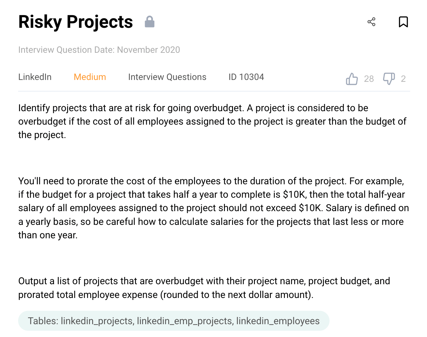
Link to the question: https://platform.stratascratch.com/coding/10304-risky-projects
The problem uses three tables: linkedin_projects, linkedin_emp_projects, linkedin_employees
The table linkedin_projects has the following fields.
| id: | int |
| title: | varchar |
| budget: | varchar |
| start_date: | datetime |
| end_date: | datetime |
The dataset linkedin_emp_projects contains the following fields.
| emp_id: | int |
| project_id: | int |
The dataset linkedin_employees with the following fields
| id: | int |
| first_name: | varchar |
| last_name: | varchar |
| salary: | int |
Solution
This is a lengthier problem compared to the previous one. Let us break down our solution into individual smaller portions. Our plan would be
- Start off by finding the daily cost for each employee
- Then aggregate the daily cost at the project level
- Calculate the projected costs for the project by multiplying the aggregate daily cost of the project by the duration of the project
- Output the relevant results.
Let us start off by finding the daily cost. Since the salary of an employee is for a full year, we calculate the daily cost by dividing the salary by 365. Note, since the salary field is an integer, we need to convert either the numerator or denominator to a floating point to avoid integer division.
SELECT
*, salary * 1.0 / 365 AS daily_cost
FROM linkedin_employees
;
We can also accomplish the same by dividing by 365.0
SELECT
*, salary / 365.0 AS daily_cost
FROM linkedin_employees
;
We get the following output.

Next, we calculate the daily costs for each project by aggregating the employee costs for all employees associated with the project. To do this, we merge the linkedin_emp_projects table with the linkedin_employees table.
SELECT
    lep.project_id
    , SUM(le.salary / 365.0) AS daily_cost
FROM
linkedin_emp_projects AS lep
LEFT JOIN linkedin_employees AS le
    ON lep.emp_id = le.id
GROUP BY 1
;
We get the following output.
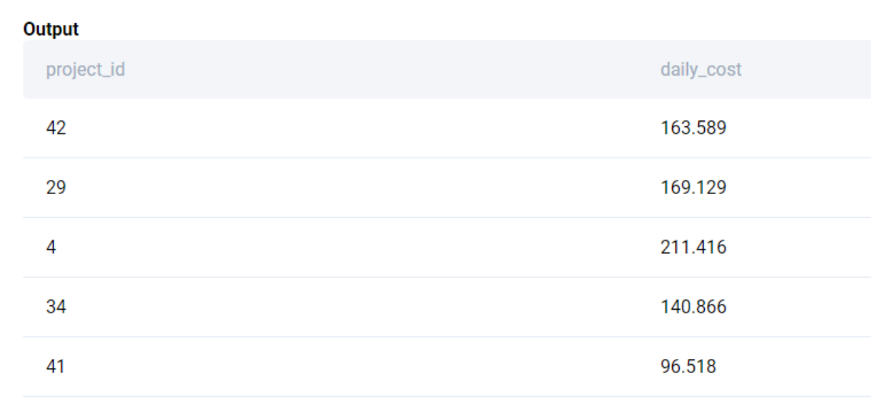
We then merge the above output with linkedin_projects to get the project details.
SELECT
    lp.title
    , lp.budget
    , lp.start_date
    , lp.end_date
    , SUM(le.salary / 365.0) AS daily_cost
FROM
linkedin_projects AS lp
LEFT JOIN linkedin_emp_projects AS lep
    ON lp.id = lep.project_id
LEFT JOIN linkedin_employees AS le
    ON lep.emp_id = le.id
GROUP BY 1,2,3,4
;
We get the following output.
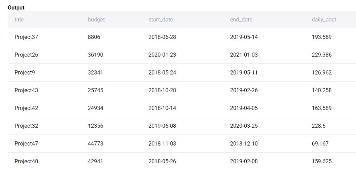
Now we have all the data in a single table. We can now calculate the projected costs based on the number of days between start_date and end_date and multiply it with the daily costs.
WITH merged AS (
SELECT
    lp.title
    , lp.budget
    , lp.start_date
    , lp.end_date
    , SUM(le.salary / 365.0) AS daily_cost
FROM
linkedin_projects AS lp
LEFT JOIN linkedin_emp_projects AS lep
    ON lp.id = lep.project_id
LEFT JOIN linkedin_employees AS le
    ON lep.emp_id = le.id
GROUP BY 1,2,3,4
)
SELECT
    title
    , budget
    , (end_date - start_date)::INT * daily_cost AS projected_cost
FROM merged
;
We get the following output.
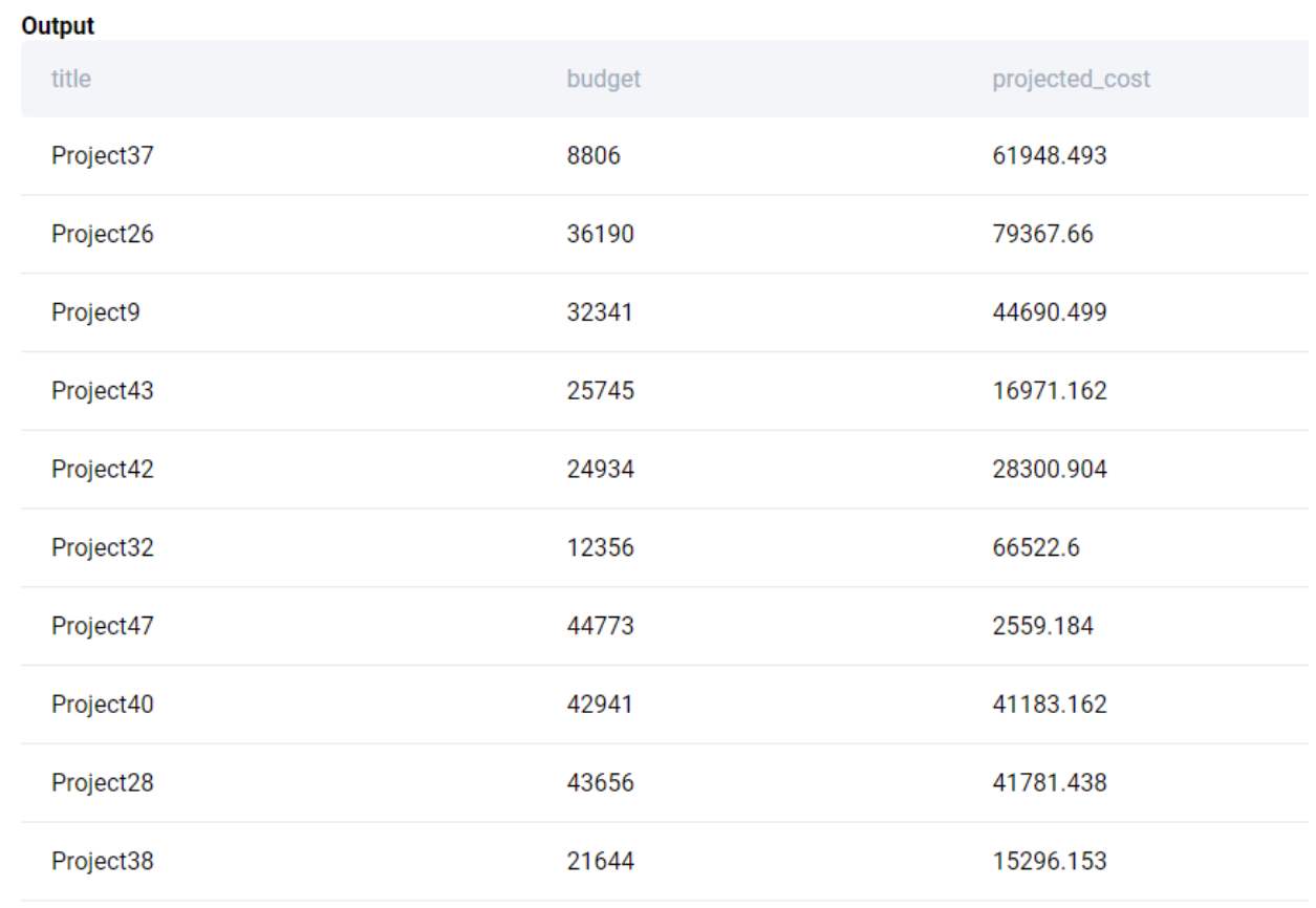
We finally round up the projected_cost and output only those projects where the projected_cost is more than the budget.
WITH merged AS (
SELECT
    lp.title
    , lp.budget
    , lp.start_date
    , lp.end_date
    , SUM(le.salary / 365.0) AS daily_cost
FROM
linkedin_projects AS lp
LEFT JOIN linkedin_emp_projects AS lep
    ON lp.id = lep.project_id
LEFT JOIN linkedin_employees AS le
    ON lep.emp_id = le.id
GROUP BY 1,2,3,4
)
SELECT
    title
    , budget
    , CEIL((end_date - start_date)::INT * daily_cost) AS projected_cost
FROM merged
WHERE (end_date - start_date)::INT * daily_cost > budget
;
You can refer to our article “different types of SQL JOINs” to understand the concept of joins in greater detail.
Aggregation in Window Functions

The knowledge and application of window functions is what separates the top SQL Analysts from the good ones. Window functions can save a lot of time if used properly as they help save intermediate queries for aggregating and then merging back to the original dataset. This is a very common use case in the day of a Data Analyst and Data Scientist. We start off with a simple problem from an Amazon Data Science Interview.
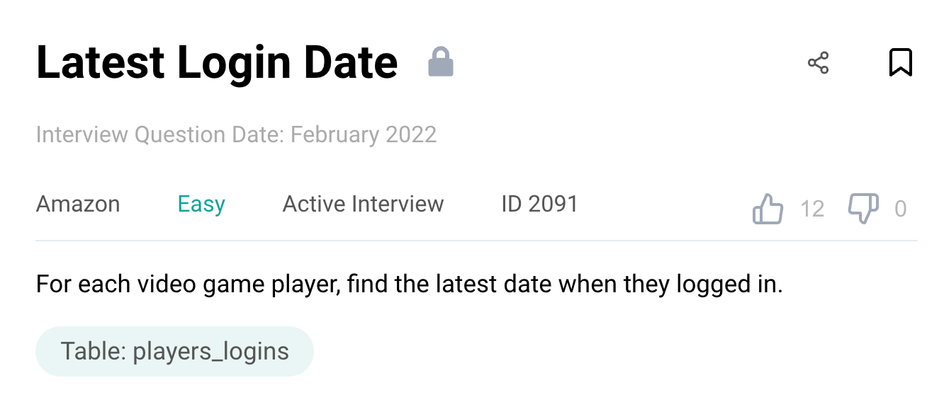
Question #6: Latest Login Date
Find the latest date that each video game player logged in.
Link to the question: https://platform.stratascratch.com/coding/2091-latest-login-date
The problem uses the players_logins table with the following fields
| player_id: | int |
| login_date: | datetime |
Solution
This problem can be solved very easily by using MAX() in the GROUP BY clause.
SELECT
    player_id
    , MAX(login_date) AS latest_login
FROM players_logins
GROUP BY 1
;
But let us solve this slightly differently. This will help us understand how the aggregation works in window functions. We need to find the latest login date, partitioning over the player_id.
SELECT
    player_id
    , login_date
    , MAX(login_date) OVER (PARTITION BY player_id) AS latest_login
FROM players_logins
;
We get the following output.
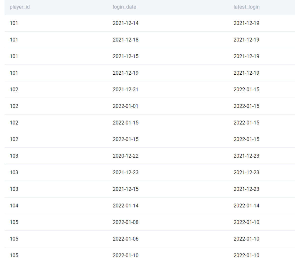
We have the latest login for each player, we can simply remove the duplicates by using the DISTINCT clause to get the final output.
SELECT
    DISTINCT
    player_id
    , MAX(login_date) OVER (PARTITION BY player_id) AS latest_login
FROM players_logins
;
The advantage of using a window function versus a GROUP BY earlier is that we add a field with the latest login date for each player in a single query call. We did not have to separately aggregate the metric and merge it back to the original dataset. This can help us compare the aggregate metric with the individual values. Something that will be very useful in the next problem. This one is from a Netflix Data Science Interview.
Question #7: Difference in Movie Ratings
For each actor, report the difference of the average lifetime rating across all movies from the rating received in the last but one movie that she acted in. Consider only the movies where the role type is ‘Normal Acting’. The id field is a sequential ID created based on the chronological order of the movies that were released. Exclude the roles that have no ratings.
Output the actor name, lifetime rating, rating of the penultimate movie, and the absolute difference between the two ratings.
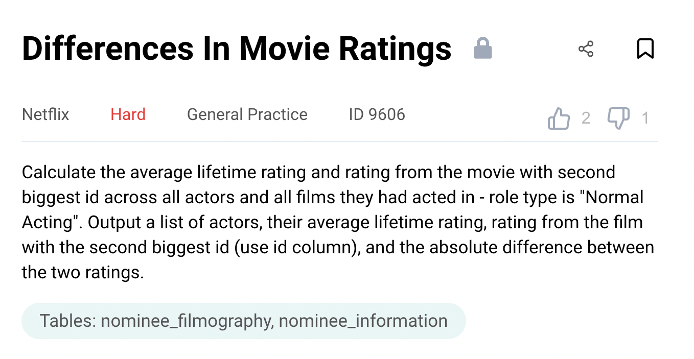
Link to the question: https://platform.stratascratch.com/coding/9606-differences-in-movie-ratings
The problem uses two tables - nominee_filmography and nominee_information. The table nominee_filmography has the following fields.
| name: | varchar |
| amg_movie_id: | varchar |
| movie_title: | varchar |
| role_type: | varchar |
| rating: | float |
| year: | int |
| id: | int |
The table nominee_information has the following fields.
| Unnamed: 0: | int |
| name: | varchar |
| amg_person_id: | varchar |
| top_genre: | varchar |
| birthday: | datetime |
| id: | int |
Solution
If one reads this SQL aggregate functions interview question carefully, we do not need the second table. All the data that we need is present in the first table (nominee_filmography) itself. We can solve the problem in the following manner
- Find the average rating for all the movies that an actor has acted in.
- Find the rating for the penultimate movie for each actor
- Report the difference between the two and output the relevant fields.
We need to exclude those movies where there is no rating provided and include only those movies where the role type is ‘Normal Acting’. We start off by finding the average rating. Instead of using a GROUP BY clause, we use a window function since we will be using a window function for the second step as well.
SELECT
    name
    , id
    , rating
    , AVG(rating) OVER (PARTITION BY name) AS avg_rating
FROM nominee_filmography
WHERE role_type = 'Normal Acting'
AND rating IS NOT NULL
;
We get the following output.
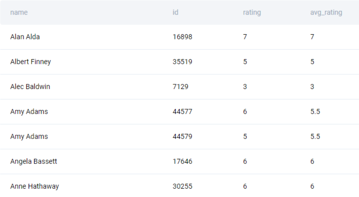
Now we add another window function to calculate the rank of the movie based on the id field.
SELECT
    name
    , id
    , rating
    , AVG(rating) OVER (PARTITION BY name) AS avg_rating
    , RANK() OVER (PARTITION BY name ORDER BY id DESC) AS movie_order
FROM nominee_filmography
WHERE role_type = 'Normal Acting'
AND rating IS NOT NULL
;
We get the following output.
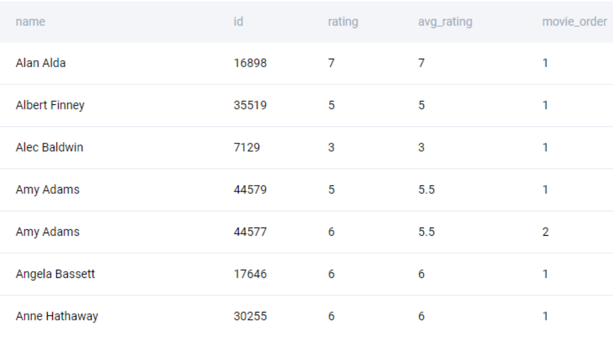
We now have the overall movie rating and the rank of the movie (as per release date) for each movie that an actor acted in. Now we simply find the movie ranked 2 (the penultimate movie) and find the absolute difference from the average rating.
SELECT
    name
    , avg_rating
    , rating
    , ABS(avg_rating - rating) AS difference
FROM (
    SELECT
        name
        , id
        , rating
        , AVG(rating) OVER (PARTITION BY name) AS avg_rating
        , RANK() OVER (PARTITION BY name ORDER BY id DESC) AS movie_order
    FROM nominee_filmography
    WHERE role_type = 'Normal Acting'
    AND rating IS NOT NULL
    ) AS ranked
WHERE movie_order = 2
;
You can read our full-blown guide on window functions here.
Bonus Text Aggregation

Let us finish off our look at aggregations by applying aggregate functions to text manipulation. With unstructured data becoming increasingly common, it is important that we get comfortable using text manipulation functions in SQL. We have an article dedicated specifically to text manipulation here in case you want to know more about text-specific functions. For the purpose of this exercise, we will use a problem that came up in an Amazon Data Science Interview, which is pretty hard. But let us try to solve this in a slightly different manner.
Question #8: Player with the Longest Streak
Given the match date and the outcome of the match for table tennis players, find the longest winning streak. A winning streak is the number of consecutive matches a player has won. Output the ID(s) of player(s) with the longest streak and the length of the streak.

Link to the question: https://platform.stratascratch.com/coding/2059-player-with-longest-streak
The problem uses the players_results table with the following fields
| player_id: | int |
| match_date: | datetime |
| match_result: | varchar |
Solution
To solve this SQL aggregate functions interview question, we need to understand how a streak is defined and how we can identify them. Let us take a hypothetical sequence of wins and losses for a player.
W, W, L, L, W, L, W, W, W, L, L, L, W, W, L, W, L, W, W, L, L, L, W
If we disregard the losses, the sequence becomes something akin to this.
W, W, _ , _, W, _, W, W, W, _, _, _, W, W, _, W, _, W, W, _, _, _, W
The start and end of a steak can be identified simply by the presence of space. So in the above example, the streaks are 2,1,3,2,1,2,1. We can then take the longest of these streaks as the best streak for the player (three in our example).
To do this in SQL in the manner described above, we need to do the following.
- Concatenate all the results in the order of the match_date
- Split the result string into individual streaks by removing the intermediate losses.
- Find the length of the streak
- Aggregate at player level keeping the longest streak for each player
- Output the longest streak along with the player(s) with the longest streak.
We start off by concatenating the result of each match in chronological order by player.
SELECT
    player_id
    , string_agg(match_result, '' ORDER BY match_date) as result_string
FROM players_results
GROUP BY 1
;
We get the following
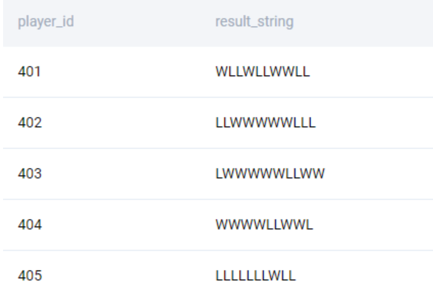
We then proceed to split the strings. To do this, we use the string_to_array function and convert the result string into an array by using ‘L’ as the delimiter.
SELECT
    player_id
    , string_to_array(string_agg(match_result, '' ORDER BY match_date), 'L') as win_streak
FROM players_results
GROUP BY 1
We get an array of streaks.
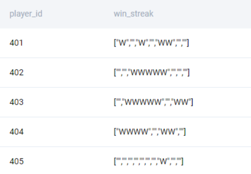
All we need to do is use the blanks to identify the start and end of the streaks. Now we proceed to split the array to individual streaks. To do this, we use the UNNEST() function.
SELECT
    player_id
    , unnest(string_to_array(string_agg(match_result, '' ORDER BY match_date), 'L')) as win_streak
FROM players_results
GROUP BY 1
;
We now have individual streaks as below.
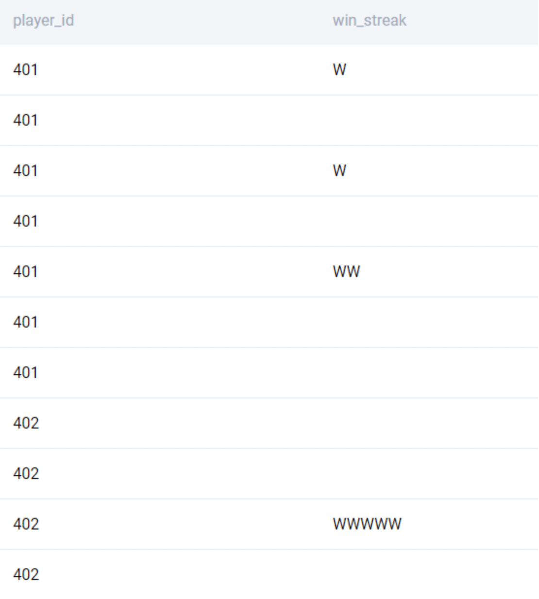
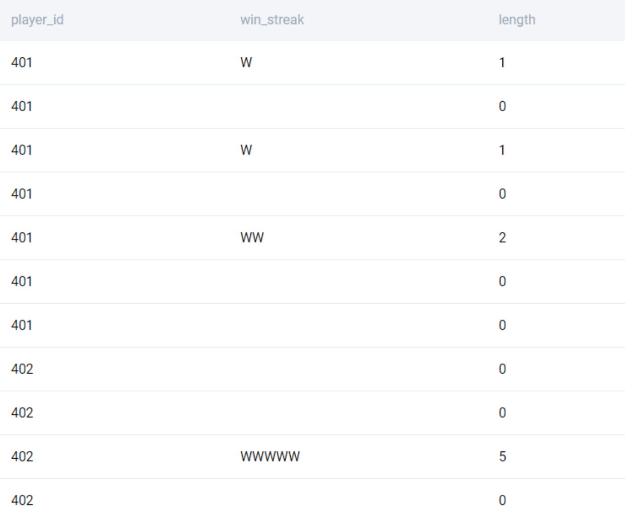
The problem has now been reduced to finding the length of the longest ‘win_streak’. This can be done by using the LENGTH() function.
WITH res_str AS (
    SELECT
        player_id
        , unnest(string_to_array(string_agg(match_result, '' ORDER BY match_date), 'L')) as win_streak
    FROM players_results
    GROUP BY 1
)
SELECT
    player_id
    , win_streak
    , length(win_streak)
FROM res_str
;
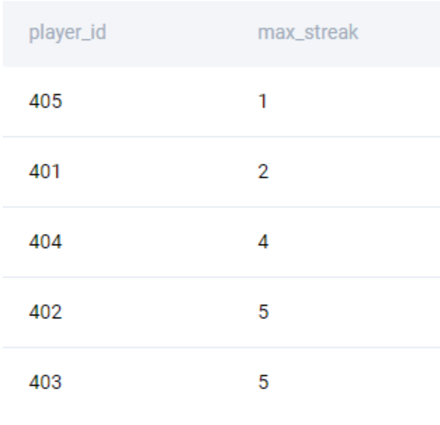
We then aggregate at a player level by using the GROUP BY clause.
WITH res_str AS (
    SELECT
        player_id
        , unnest(string_to_array(string_agg(match_result, '' ORDER BY match_date), 'L')) as win_streak
    FROM players_results
    GROUP BY 1
)
SELECT
    player_id
    , MAX(length(win_streak)) as max_streak
FROM res_str
GROUP BY 1
;
And then use a window function as earlier to find the player(s) with the longest streak.
WITH res_str AS (
    SELECT
        player_id
        , unnest(string_to_array(string_agg(match_result, '' ORDER BY match_date), 'L')) as win_streak
    FROM players_results
    GROUP BY 1
), ranked_streaks AS (
    SELECT
        player_id
        , MAX(length(win_streak)) as max_streak
        , RANK() OVER (ORDER BY MAX(length(win_streak)) DESC) as rnk
    FROM res_str
    GROUP BY 1
)
SELECT
    player_id
    , max_streak
FROM ranked_streaks
WHERE rnk = 1
;
You can know more about STRING_AGG in detail here.
Conclusion
In this article we looked at the various application of aggregations in SQL. We started with aggregating the entire dataset and then applied aggregations to sub-groups using the GROUP BY clause and finally finished off with aggregations in windowing functions. We also looked at an example of text aggregation. With the size of data increasing manifold every day, it is critical for Data Analysts and Data Scientists to master aggregation functions. As with every other skill in life, all it takes is practice, patience, and persistence to master. Sign up today for a free account on StrataScratch and join over 20,000 other like-minded professionals aspiring to crack their next Data Science Interview at top companies like Netflix, Amazon, Microsoft, Apple, et al.
Share


