Python Pandas Interview Questions for Data Science

Categories:
 Written by:
Vivek Sankaran
An overview of the basics of data manipulation and the types of Python Pandas interview questions asked in Data Science Interviews.
Pandas is the most common library for manipulating tabular data. Think of it like a spreadsheet or SQL table within Python. One can manipulate structured data just as one will be using Excel or Google Sheets. A lot of machine learning and allied libraries like SciPy, Scikit-learn, Statsmodels, NetworkX etc. and visualization libraries like Matplotlib, Seaborn, Plotly et al work very well with Pandas Data Structures. A lot of specialized libraries like geo-pandas, quandl, Bokeh, et al have been built on top of the Pandas Library. Many proprietary libraries used for algorithmic trading, data analysis, ETL processes, etc use Pandas extensively.
The Pandas library has been developed since 2010, hence there is a well documented code available. You can go through the documentation here. This versatility, flexibility and convenience makes Pandas the go to solution for working with Machine Learning Data. If you are serious about appearing for Python Data Science Interviews, proficiency in Pandas is the bare minimum expectation.
Technical Concepts tested in Python Pandas Interview Questions
The problems involving Pandas can be broadly grouped into the following categories.
- Sorting DataFrames
- Handling Duplicates
- Aggregations
- Merging DataFrames
- Calculated Fields
- Datetime Operations
- Text Manipulation
- Offsets
- Applying functions
In this article we will start with the basics and cover the first five areas. The remaining areas are covered in the second part of the series. Check out the second part here.
Pandas Basics
Before we start working on different functionalities available in the Pandas library, we need to understand how Pandas organizes its data. This will help us understand the operations performed in detail. Please note that our aim for this article is understanding the workings of Pandas not code-optimization, hence we have chosen relatively easier data sets. We will be handling complex datasets and trickier problems in the next article in this series.
We use a simple dataset tracking Covid-19 data in India. We start off by looking at how the data looks like
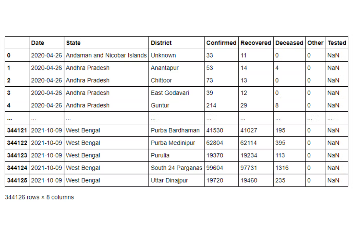
Pandas organizes the data in form of a two-dimensional data structure called DataFrame
This is very similar to a Spreadsheet or a SQL table. Here is a rough analogy of the various terms.
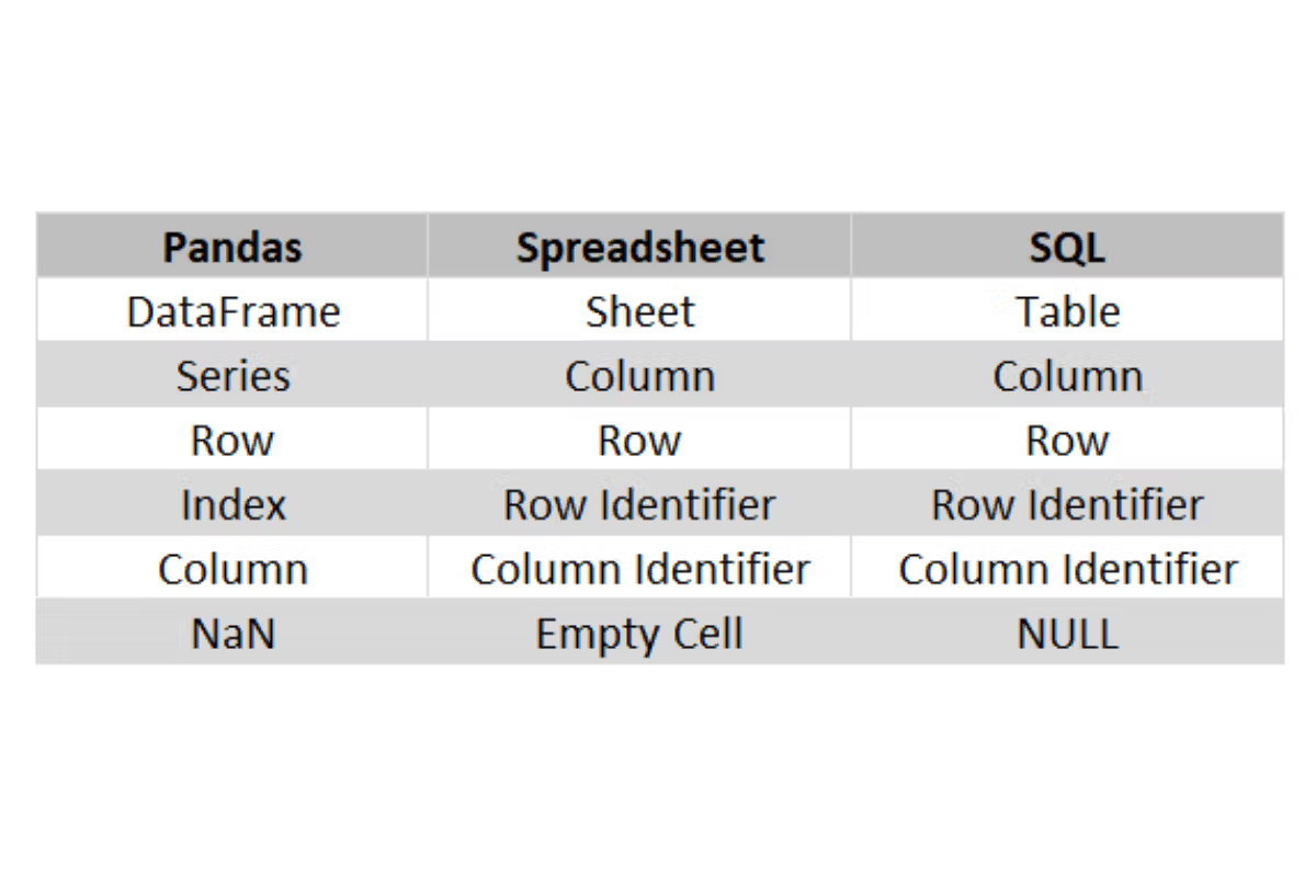
We can find the basic information about the DataFrame using the info method.
covid_df.info()<class 'pandas.core.frame.DataFrame'>
RangeIndex: 344126 entries, 0 to 344125
Data columns (total 8 columns):
# Column Non-Null Count Dtype
--- ------ -------------- -----
0 Date 344126 non-null datetime64[ns]
1 State 344126 non-null object
2 District 344126 non-null object
3 Confirmed 344126 non-null int64
4 Recovered 344126 non-null int64
5 Deceased 344126 non-null int64
6 Other 344126 non-null int64
7 Tested 258862 non-null float64
dtypes: datetime64[ns](1), float64(1), int64(4), object(2)
memory usage: 21.0+ MB
Each of the column names is the identifier for a column. Similar to what one will get in an SQL table. Just as with an SQL table, we can change the column names using the rename() method.
Where DataFrames differ from a SQL table or an Excel Sheet is in flexibility of the row identifiers – The index. At present, the index contains sequential values just as with SQL Tables or a Spreadsheet. However, we can create our own row values and they need not be unique or sequential. For example, we can set the State Column to be the index using the set_index() method.
state_idx = covid_df.set_index('State')
state_idx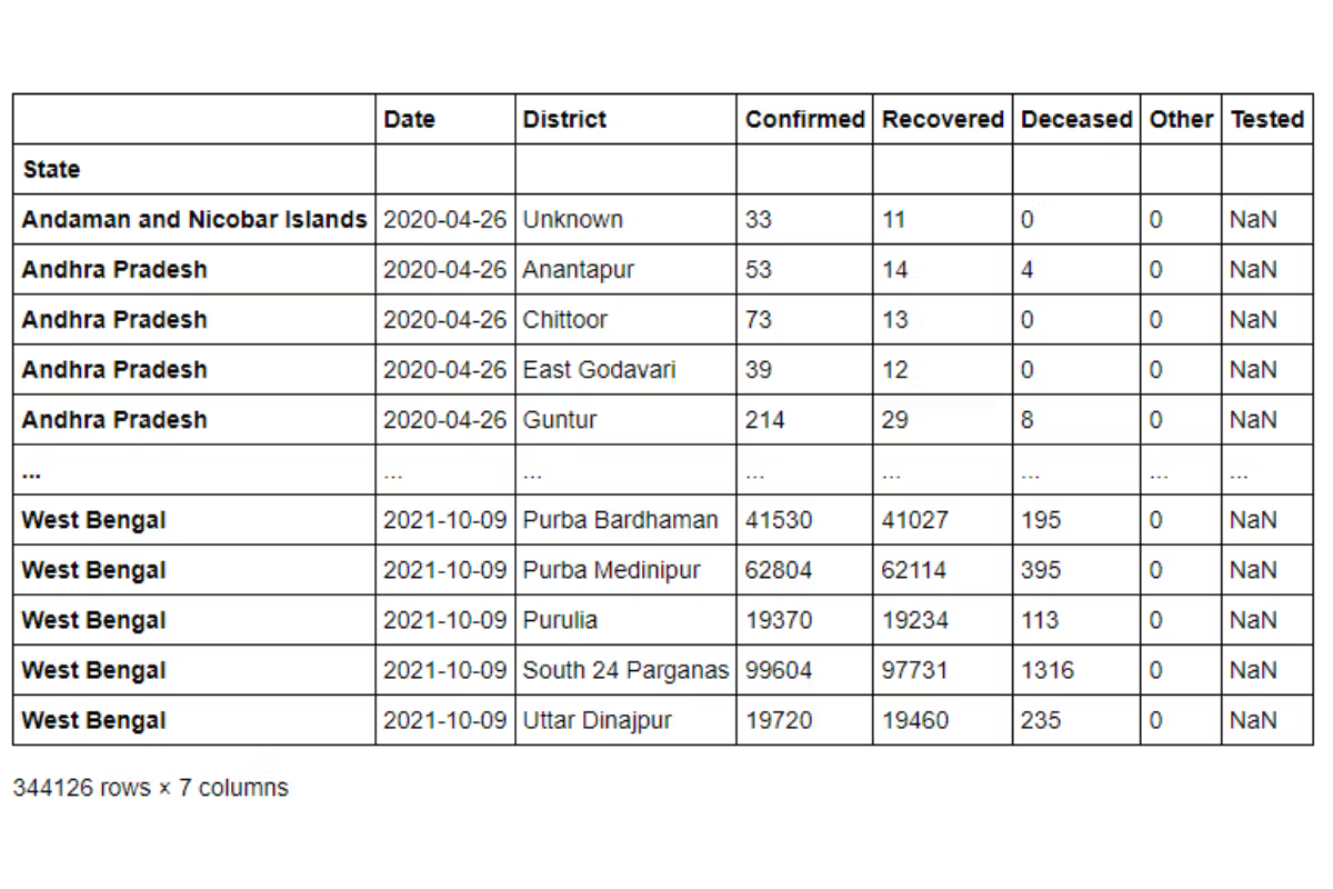
The state field is no longer considered a column. When we call the info() method on the new DataFrame, we can see that the state column from our older dataset is now set as the index.
<class 'pandas.core.frame.DataFrame'>
Index: 344126 entries, Andaman and Nicobar Islands to West Bengal
Data columns (total 7 columns):
 #   Column     Non-Null Count   Dtype
---  ------     --------------   -----
 0   Date       344126 non-null  datetime64[ns]
 1   District   344126 non-null  object
 2   Confirmed  344126 non-null  int64
 3   Recovered  344126 non-null  int64
 4   Deceased   344126 non-null  int64
 5   Other      344126 non-null  int64
 6   Tested     258862 non-null  float64
dtypes: datetime64[ns](1), float64(1), int64(4), object(1)
memory usage: 21.0+ MB
We can get back a sequential Index by calling the reset_index() method.
Each column of data in a Pandas DataFrame is referred to as a Pandas Series. Every time we access a Pandas Series, we also get the index along. Example, if we take the District Series, we will get a column with State field as the index.
state_idx['District']State
Andaman and Nicobar Islands Unknown
Andhra Pradesh Anantapur
Andhra Pradesh Chittoor
Andhra Pradesh East Godavari
Andhra Pradesh Guntur
...
West Bengal Purba Bardhaman
West Bengal Purba Medinipur
West Bengal Purulia
West Bengal South 24 Parganas
West Bengal Uttar Dinajpur
Name: District, Length: 344126, dtype: object
This can help us in subsetting the data in a lot of ways that are not available with Spreadsheets or SQL Tables.
Some very useful DataFrame functions that can be used to explore the data quickly are
.head() : This method shows n observations from the start of the DataFrame. If no argument is passed, then by default it returns the first 5 rows.
covid_df.head(20)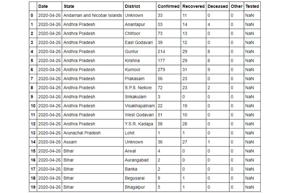
tail() : similar to the head() method, but this will give the last n rows of the DataFrame. If no argument is passed, then by default it returns the last five rows.
value_counts() : this gives us the frequency distribution of the values.
covid_df['State'].value_counts()Uttar Pradesh 39738
Madhya Pradesh 27409
Tamil Nadu 21173
Bihar 20115
Rajasthan 19594
Maharashtra 19115
Gujarat 18044
Karnataka 16290
Odisha 16083
Chhattisgarh 14918
Arunachal Pradesh 12944
West Bengal 12581
Jharkhand 12497
Haryana 11872
Punjab 11695
Jammu and Kashmir 10596
Andhra Pradesh 7950
Kerala 7449
Uttarakhand 6790
Himachal Pradesh 6225
Nagaland 5717
Mizoram 5377
Meghalaya 5359
Tripura 4160
Puducherry 2063
Dadra and Nagar Haveli and Daman and Diu 1495
Assam 1421
Ladakh 1064
Manipur 962
Andaman and Nicobar Islands 532
Telangana 532
Goa 532
Delhi 532
Chandigarh 532
Sikkim 505
Lakshadweep 265
Name: State, dtype: int64
Note: it will ignore missing values in the frequency count. So, if you want to include missing values, set the dropna argument to False. In this case, there were no missing values so we omitted this argument.
Sorting
As with SQL and Spreadsheets, we can sort the table based on a column or a sequence of columns. By default the values are sorted in ascending order, we can change the order by changing the ascending parameter. Example we can sort our Covid Dataset by the descending order of the State Names but Ascending order of the District Names.
covid_df.sort_values(by = ['State', 'District'], ascending = [False, True])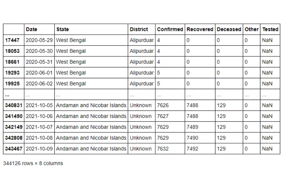
Duplicates
Dealing with duplicates is a very common problem encountered in Data Science Interview questions. The presence of duplicates need not mean incorrect data. For example, a customer might purchase multiple items, hence the transaction data might contain repeated values of the same card number or customer id. Pandas provides a convenient way of dropping duplicates and creating a unique set of records. Once can apply the drop_duplicates() method for this purpose.
Suppose we want to find the list of distinct states from our Covid Dataset. We can do it using passing the entire series to a Python set and then converting it back into a Pandas Series. Conversely, we can apply the drop_duplicates() method. We can either apply it to the Pandas Series,
covid_df['State'].drop_duplicates()or on the entire dataset and specify a subset to remove duplicates from.
covid_df.drop_duplicates(subset = ['State'])['State']0 Andaman and Nicobar Islands
1 Andhra Pradesh
13 Arunachal Pradesh
14 Assam
15 Bihar
37 Chandigarh
38 Chhattisgarh
43 Delhi
44 Goa
45 Gujarat
75 Himachal Pradesh
81 Haryana
101 Jharkhand
111 Jammu and Kashmir
128 Karnataka
149 Kerala
163 Ladakh
165 Maharashtra
198 Meghalaya
199 Manipur
200 Madhya Pradesh
227 Mizoram
228 Odisha
238 Punjab
257 Puducherry
259 Rajasthan
290 Telangana
291 Tamil Nadu
328 Tripura
330 Uttar Pradesh
388 Uttarakhand
394 West Bengal
3979 Dadra and Nagar Haveli and Daman and Diu
11267 Nagaland
13703 Sikkim
170212 Lakshadweep
Name: State, dtype: object
Let us try to apply this in one of the Python Pandas interview questions. This one came up in an AirBnB Data Science Interview.
Python Pandas Interview Questions

Find all neighborhoods present in this dataset
Find all neighbourhoods present in this dataset.
Link to the question: https://platform.stratascratch.com/coding/9626-find-all-neighborhoods-present-in-this-dataset
The problem uses the airbnb_search_details dataset that has the following fields.
| id | int64 |
| price | float64 |
| property_type | object |
| room_type | object |
| amenities | object |
| accommodates | int64 |
| bathrooms | int64 |
| bed_type | object |
| cancellation_policy | object |
| cleaning_fee | bool |
| city | object |
| host_identity_verified | object |
| host_response_rate | object |
| host_since | datetime64[ns] |
| neighbourhood | object |
| number_of_reviews | int64 |
| review_scores_rating | float64 |
| zipcode | int64 |
| bedrooms | int64 |
| beds | int64 |
The dataset looks something like this.
Approach and Solution
This is a relatively straightforward problem. We simply need to drop the duplicates on the neighborhood column. As earlier, we can either apply the drop_duplicates() method on the entire dataset and then report the series. Or we can take the series and then drop the duplicates.
# Import your libraries
import pandas as pd

# Take the relevant series and apply the drop_duplicates() method
airbnb_search_details['neighbourhood'].drop_duplicates()
And we get our required solution.
Slicing Pandas Dataset
We can use a subset of the DataFrame instead of the full set. If you want only particular columns from the dataset, one can simply pass the list of relevant columns into the slicer.
covid_df[['Date','State', 'District', 'Confirmed']]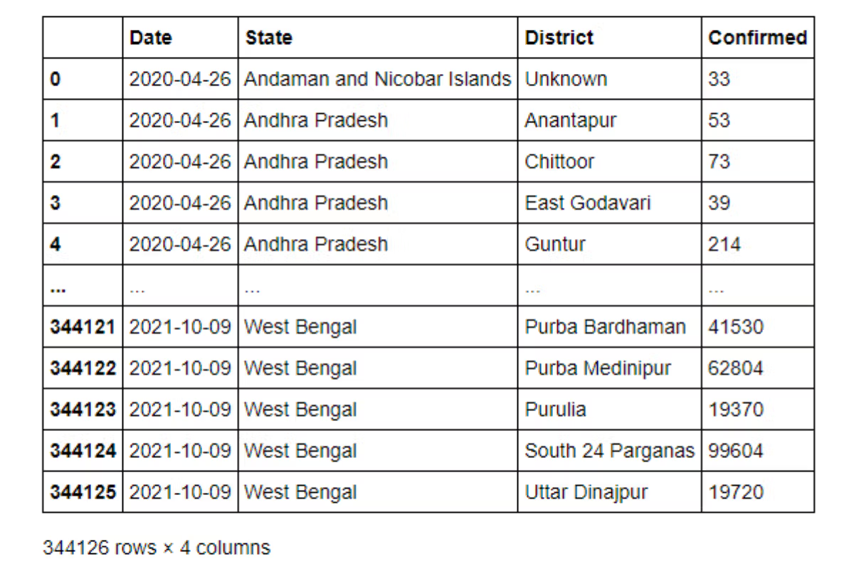
Note you must use two sets of square brackets. If we use only a single square bracket, Pandas will assume that you want to create a Series. But a series will have only one field and therefore it will give an error.
You can also subset specific rows based on their values, like the WHERE condition in SQL or Filter option in Spreadsheets. Suppose we want only data from the states of Goa and Maharashtra. We can simply pass this as a condition and slice the DataFrame as one would slice a string or a list.
covid_df[(covid_df['State'] == 'Goa' )| (covid_df['State'] == 'Maharashtra')]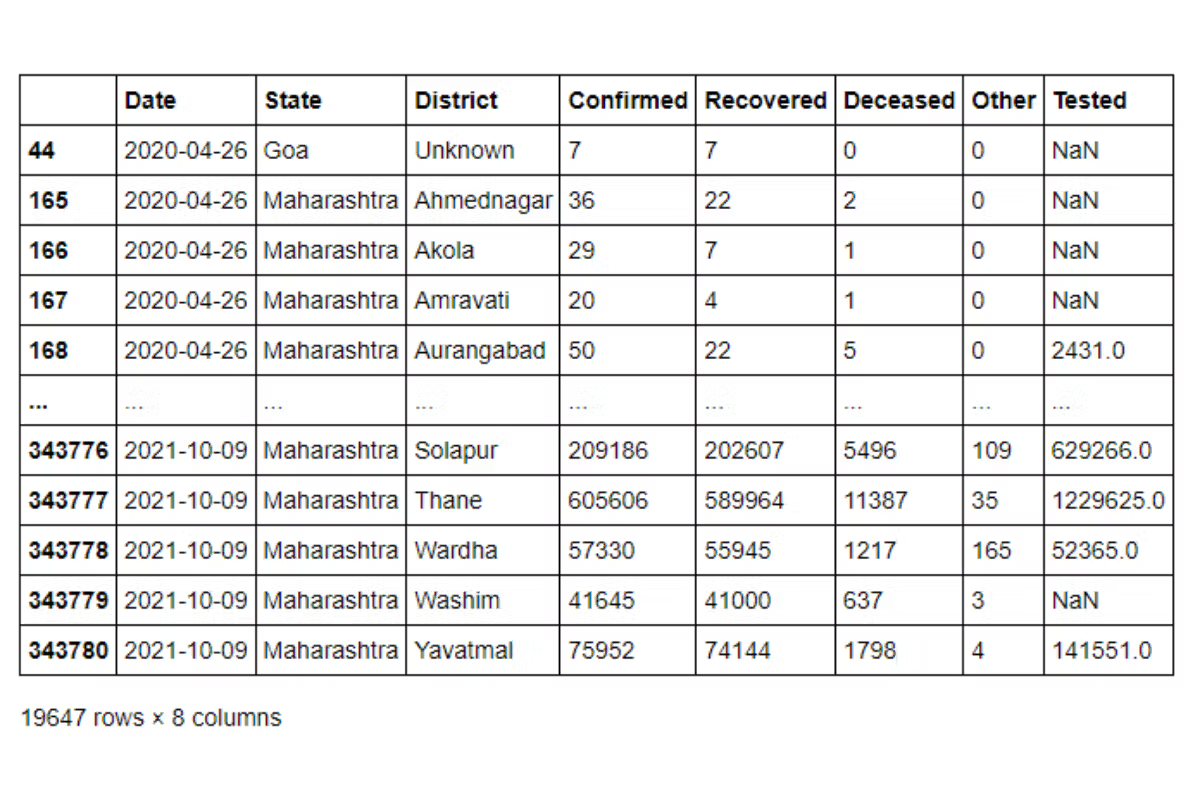
Let us see what happens under the hood. The DataFrame slicer uses a Boolean Masking array. The condition inside the slicer returns a Boolean Series.
(covid_df['State'] == 'Goa' )| (covid_df['State'] == 'Maharashtra')0 False
1 False
2 False
3 False
4 False
...
344121 False
344122 False
344123 False
344124 False
344125 False
Name: State, Length: 344126, dtype: bool
When we pass this into the slicer, only the rows with True are retained. This is a very efficient and powerful way of filtering data.
Let us use this in a real-life Python Pandas interview question. This problem is from a Spotify Data Science Interview.
Top 10 Ranked Songs
Report the top 10 ranked songs by position. Output the track and the ranks in the descending order of ranks. If there are multiple songs with the same rank, sort them in alphabetical order of the track name.
Find the top 10 ranked songs by position. Output the track name along with the corresponding position and sort records by the position in descending order and track name alphabetically, as there are many tracks that are tied for the same position.
Link to the question: https://platform.stratascratch.com/coding/9995-top-10-ranked-songs
The problem uses the spotify_worldwide_daily_song_ranking dataset that has the following fields.
| id | int64 |
| position | int64 |
| trackname | object |
| artist | object |
| streams | int64 |
| url | object |
| date | datetime64[ns] |
| region | object |
This is what the dataset looks like.
Approach and solution
To solve this problem, we first subset the songs that are ranked 10 or better.
# Import your libraries
import pandas as pd

# get the top10 songs
top10_songs = spotify_worldwide_daily_song_ranking[spotify_worldwide_daily_song_ranking['position'] <=10]
The output looks like this

Now we need to sort this in descending order of position, ascending order of trackname and output the relevant fields.
# Sort and output relevant fields
top10_songs.sort_values(by = ['position', 'trackname'], ascending = [False, True])[['trackname','position']]
The output looks like this.
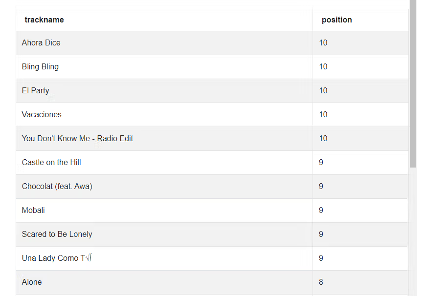
The problem is not over since we might have duplicate records as a song might be ranked No 1 in multiple locations. To remove duplicate records, we can simply call the drop_duplicates() method on the output.
# Sort and output relevant fields
top10_songs.sort_values(by = ['position', 'trackname'], ascending = [False, True])[['trackname','position']].drop_duplicates()
And we have the desired output now.
Aggregations
A very common test area in Python Pandas interview questions is aggregations or rollups. Business professionals want a top-level overview of the metrics before digging down deeper into sub-segments. Aggregations are very handy in these situations. These are similar to a Pivot Table in a spreadsheet or Group By methods in SQL. Pandas provides many ways to create these aggregations. In this article we look at the most basic one – the groupby method.
Let’s say we wanted to find the average number of confirmed cases reported in each district. We can do this by passing the State and District combination as the grouper variables and then calculate the average by calling the mean() method.
covid_df.groupby(['State', 'District']).mean()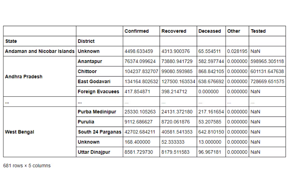
As you can see from the result, the State and District combination now becomes an index. In Pandas this is called a Multi-Index Data. You can easily get the index values back into the DataFrame by calling the reset_index() method. Or you can prevent the creation of this index by setting the as_index argument to False in the groupby method.
covid_df.groupby(['State', 'District'], as_index = False).mean()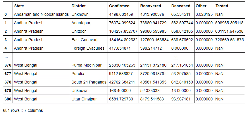
This gives us the grouper variable as columns in the DataFrame and we can use them for further analysis without having to resort to reset_index() again and again. Further, you would have noticed that Pandas calculates the mean of all numeric variables. We can retain the relevant columns by subsetting the final dataset. Or we can simply call the agg() method on a grouped DataFrame.
covid_df.groupby(['State', 'District'], as_index = False).agg
({'Confirmed' : 'mean'})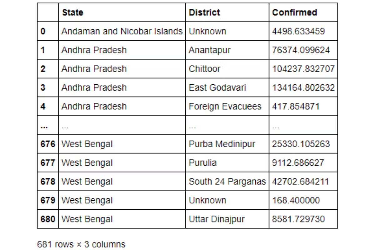
The agg() method is also advantageous in calculating multiple values aggregates at the same time. Suppose We want to report not only the average of the confirmed cases. but also, the maximum number of deaths, we can pass these as a dictionary to the agg() method.
covid_df.groupby(['State', 'District'], as_index = False).agg
({'Confirmed' : 'mean', 'Deceased' : 'max'})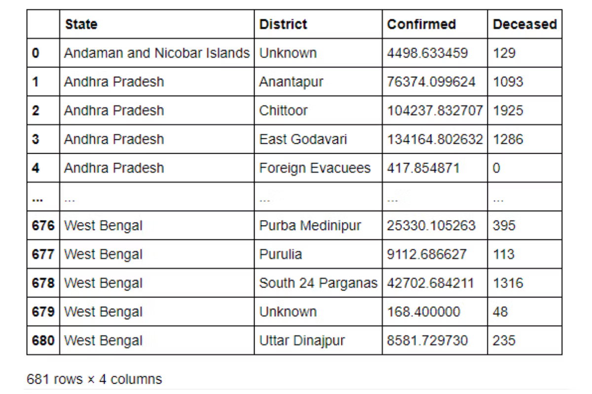
Let us try to use this in one of the Python Pandas interview questions. This one is from an AirBnB Data Science Interview.
Cheapest Properties
Find the price of the cheapest property for every city.
Last Updated: January 2018
Find the price of the cheapest property for every city.
Link to the question: https://platform.stratascratch.com/coding/9625-cheapest-properties
This problem uses the airbnb_search_details that we had seen in an earlier problem. Let us recap the fields present.
| id | int64 |
| price | float64 |
| property_type | object |
| room_type | object |
| amenities | object |
| accommodates | int64 |
| bathrooms | int64 |
| bed_type | object |
| cancellation_policy | object |
| cleaning_fee | bool |
| city | object |
| host_identity_verified | object |
| host_response_rate | object |
| host_since | datetime64[ns] |
| neighbourhood | object |
| number_of_reviews | int64 |
| review_scores_rating | float64 |
| zipcode | int64 |
| bedrooms | int64 |
| beds | int64 |
And this is what the data looks like.
Approach and Solution
This problem can be solved easily with the groupby method. We simply need to roll-up at city level and find the minimum of the prices column.
# Import your libraries
import pandas as pd

# Calculate the mininum prices at city level
airbnb_search_details.groupby(by = ['city'], as_index = False).agg({'price': 'min'})
Merging
Till now we have used only a single dataset. However real life dataset are optimized by splitting them into different tables. Pandas supports multiple ways of combining multiple datasets. We can stack one DataFrame on top of another or alongside other using the append() and concat() methods. Or we can use an SQL style merge using the merge() merge method. Let us see how to use the merge method using a SalesForce Python Pandas interview question.
Average Salaries
Report the department, first name and salary of each employee along with the average salary of the corresponding department.
Last Updated: May 2019
Compare each employee's salary with the average salary of the corresponding department. Output the department, first name, and salary of employees along with the average salary of that department.
Link to the question: https://platform.stratascratch.com/coding/9917-average-salaries
This problem uses the employee dataset which has the following fields.
| id | int64 |
| first_name | object |
| last_name | object |
| age | int64 |
| sex | object |
| employee_title | object |
| department | object |
| salary | int64 |
| target | int64 |
| bonus | int64 |
| object | |
| city | object |
| address | object |
| manager_id | int64 |
The dataset looks like this.
Approach and Solution
To solve this Python Pandas interview question we need to find the average salary of each department and add that field to the DataFrame. We start off by calculating the average salaries using the groupby method. We also rename the salary field so that the names do not conflict during merge. Note this will not result in an error, but the names will be suffixed with identifiers. We can change those, but to make life easier, we just rename one of the variables.
# Import your libraries
import pandas as pd

# Calculate Average Salary for each department
avg_sal = employee.groupby(by = ['department'], as_index = False).agg({'salary' : 'mean'}).rename(columns = {'salary' : 'average_salary'})
The aggregated dataset looks like this.

We now proceed to merge this back to the original DataFrame on the department field. While merging we pass only the relevant columns from the original DataFrame.
# Merge with the relevant fields from the original DataFrame
pd.merge(employee[['department', 'first_name', 'salary']], avg_sal,
on = 'department', how = 'inner')
We specify inner join. If there are no missing departments, then this will give the same result as a left join or a right join or an outer join.
Calculated Fields
Till now we have used fields that were already present in the dataset. We can also create calculated fields very easily. Let us try one with our Covid dataset. Suppose we want to calculate the recovery rate (Number of Recovered Cases / Number of Confirmed Cases), then we can simply do it like this.
covid_df['Recovery Rate'] = covid_df['Recovered'] / covid_df['Confirmed']
covid_df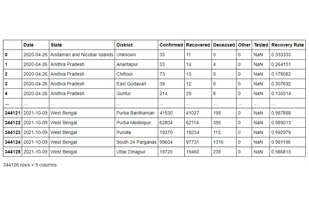
Let's use this in one of the Python Pandas interview questions. This Python Pandas interview question is from an Uber Data Science Interview.
Advertising Channel Effectiveness
Calculate the averages effectiveness for each advertising channel across the years 2017 and 2018. Report the channel and effectiveness sorted in the increasing order of effectiveness.
Advertising effectiveness is defined as the ratio of total money spent to total customers acquired.
Find the effectiveness of each advertising channel in the period from 2017 to 2018 (both included). The effectiveness is calculated as the ratio of total money spent to total customers aquired.
Output the advertising channel along with corresponding effectiveness. Sort records by the effectiveness in ascending order.
Link to the question: https://platform.stratascratch.com/coding/10012-advertising-channel-effectiveness
This problem uses the uber_advertising dataset that has the following fields.
| year | int64 |
| advertising_channel | object |
| money_spent | int64 |
| customers_acquired | int64 |
The data is present like thus.
Approach and Solution
To solve this Python Pandas interview question, we first aggregate the money_spent and customers_acquired columns across the advertising_channel. We need to ensure that we keep only the relevant years since the problem asks us to calculate these values across 2017 and 2018 only.
# Import your libraries
import pandas as pd

# Summarize the spends and customer acquired by channel
summ_df = uber_advertising[uber_advertising['year'].isin([2017, 2018])].groupby(
    by = ['advertising_channel'], as_index = False
    ).agg(
        {
            'money_spent' : 'sum', 'customers_acquired':'sum'
        }
        )
The output looks thus.
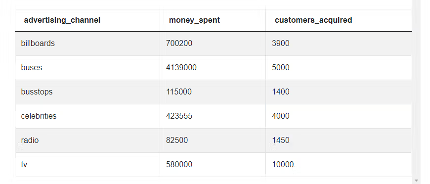
We can now calculate the effectiveness using the given formula, subset the relevant fields and sort as per the required specifications.
# Calculate effectiveness
summ_df['effct'] = summ_df['money_spent'] / summ_df['customers_acquired']
# Sort and output relevant fields
summ_df[['advertising_channel', 'effct']].sort_values(by = ['effct'])
Conclusion
In this article we looked at the basics of data manipulation with Pandas and the types of Python Pandas interview questions you can expect in any data science interview. You can find the Covid-19 dataset and the associated Python Notebook here. In the next part of this series, we will extend these concepts and look at slightly complex problems like -
- Datetime Manipulation
- Text Manipulation
- Applying Functions
- Advanced Aggregation
- Offsetting Data
- Statistics using Pandas
If you have worked with a Spreadsheet program or SQL tables, migrating to Pandas is very easy. In fact, you can use Pandas, a library to learn Python. On the StrataScratch platform, you will find over 700 coding problems and non-technical interview problems from Data Science Interviews. Check out our recent post on Top 30 Python Interview Questions and Answers. These problems are created from Data Science interviews at top companies like Netflix, Amazon, Google, Microsoft, et al. Also, check out Pandas Cheat Sheet that can help you become a better data scientist.
You can join a group of 20,000+ like minded data science aspirants to get a collaborative learning experience. Sign up for StrataScratch today and give yourself the best chance to crack interviews for the most in-demand jobs at big tech firms and start-ups across the world.
Share


