PySpark SQL Functions: Boost Big Data Processing with SQL

Categories:
 Written by:
Nathan Rosidi
Leverage PySpark SQL Functions to efficiently process large datasets and accelerate your data analysis with scalable, SQL-powered solutions.
Do you know your SQL could run ten times faster than data processing? Mixing these two with Spark SQL allows you to have a conventional (mostly known) interface like SQL and use Apache Spark to manage the heavy lifting on large-scale datasets, obtaining the best of both worlds.
In this article, we’ll review the essential PySpark SQL functions for DataFrame and some advanced ideas, such as user-defined and window functions.
What is Spark SQL?
Spark SQL is a structured data processing Spark module. It provides a basic interface for queries on structured and semi-structured data, enabling significant sharing of computational capacity.
Whether you are working with standard SQL tables or Spark SQL to handle DataFrames, the language lessens most of this hassle by allowing data to be easily retrieved with basic searches.
Core PySpark SQL Functions
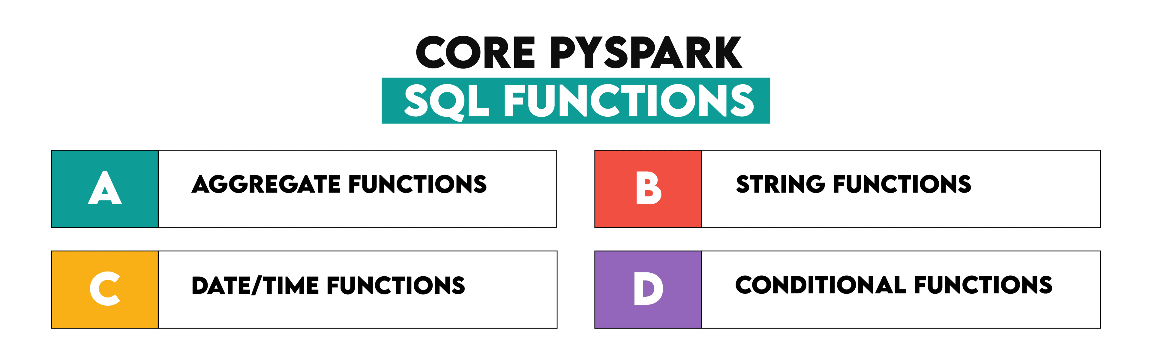
Core PySpark SQL functions include aggregate, string, date and time, and conditional functions.
Also, to know more about Pyspark, check out What Is PySpark?.
Aggregate Functions
In PySpark, SQL functions allow you to apply familiar SQL-style transformations and aggregations on large datasets.
Using built-in SQL functions, such as max() and min(), and with Column (), you can efficiently compute values like population density and identify the cities with minimum and maximum densities.
Population Density
Last Updated: January 2024
You are working on a data analysis project at Deloitte where you need to analyze a dataset containing information about various cities. Your task is to calculate the population density of these cities, rounded to the nearest integer, and identify the cities with the minimum and maximum densities. The population density should be calculated as (Population / Area).
The output should contain 'city', 'country', 'density'.
We'll focus on solving this problem using PySpark SQL functions, which will help showcase how SQL functions within PySpark can simplify real-world data analysis tasks.
Here is the link to this question above: https://platform.stratascratch.com/coding/10368-population-density
Now, let’s divide this solution into codable steps.
Step 1: Let’s load the necessary libraries.
Step 2: We filter out rows where the city area equals zero to avoid dividing by zero.
Step 3: We create a new column in the DataFram to calculate the population density.
Step 4: Then, we apply SQL functions F.max() and F.min() to find the cities with the highest and lowest densities.
Step 5: Finally, we combine both results into one DataFrame.
Here is the code.
import pyspark.sql.functions as F

cities_population = cities_population.filter(cities_population['area'] != 0)

cities_population = cities_population.withColumn('density', cities_population['population'] / cities_population['area'])

max_density_df = cities_population.filter(cities_population['density'] == cities_population.select(F.max('density')).collect()[0][0]).select('city', 'country', 'density')

min_density_df = cities_population.filter(cities_population['density'] == cities_population.select(F.min('density')).collect()[0][0]).select('city', 'country', 'density')

combined_density_df = max_density_df.union(min_density_df)

combined_density_df.toPandas()
Here is the output.
| city | country | density |
|---|---|---|
| Gotham | Islander | 5000 |
| Rivertown | Plainsland | 20 |
| Lakecity | Forestland | 20 |
The resulting DataFrame will display the city, country, and density of cities with the highest and lowest population densities. The use of SQL functions in PySpark ensures quick and efficient handling of this task, even when working with large datasets.
String Functions
PySpark has many convenient functions for handling string manipulation, transformation, and querying while dealing with type-casting.
These include functions like startswith(), substr(), and concat(), allowing you to filter, extract, and combine text. For this task, we’ll use startswith() to filter sales data for January.
Here, we will use some of them inside our interview questions from Amazon; check this one.
Top Monthly Sellers
Last Updated: January 2024
You are provided with an already aggregated dataset from Amazon that contains detailed information about sales across different products and marketplaces. Your task is to list the top 3 sellers in each product category for January. In case of ties, rank them the same and include all sellers tied for that position.
The output should contain seller_id ,total_sales ,product_category , market_place, and sales_date.
You can reach this question here: https://platform.stratascratch.com/coding/10362-top-monthly-sellers
Here is the step-by-step solution of this code:
Step 1: First, we use the startswith() function to filter the dataset for entries where the month column starts with '2024-01', which isolates January’s sales data.
Step 2: We define a window specification (Window.partitionBy()) to partition data by product categories and order them by total_sales in descending order.
Step 3: Using row_number(), we assign ranks to sellers within each product category and filter the top 3 sellers by keeping only those with a rank ≤ 3.
Here is the code to solve it:
from pyspark.sql import SparkSession
from pyspark.sql.functions import col, desc, row_number
from pyspark.sql.window import Window

january_sales = sales_data.filter(col('month').startswith('2024-01'))

window_spec = Window.partitionBy('product_category').orderBy(desc('total_sales'))

top_sellers_by_category = january_sales.withColumn('rank', row_number().over(window_spec)) \
    .filter(col('rank') <= 3) \
    .drop('rank')

top_sellers_by_category.toPandas()
Here is the output.
The resulting DataFrame will display the seller_id, total_sales, product_category, market_place, and month for the top 3 sellers in each category. Using string functions like startswith(), PySpark simplifies filtering and manipulating textual data in large-scale datasets.
Date/Time Functions
Sometimes, it is necessary to convert the timestamps to strings or concatenate them for a more user-friendly format; this can be done using functions like concat(), lit(), and cast().
In addition, you can take advantage of PySpark’s aggregation functions, such as max(), when doing time-based analysis or grouping data by some specific columns(e.g., device_type). For our case, we will find the time slot with the most active users on all device types.
Now let’s see this concept by cracking the following interview question:
Peak Online Time
Last Updated: January 2024
You are given a dataset from Amazon that tracks and aggregates user activity on their platform in certain time periods. For each device type, find the time period with the highest number of active users.
The output should contain 'user_count', 'time_period', and 'device_type', where 'time_period' is a concatenation of 'start_timestamp' and 'end_timestamp', like ; "start_timestamp to end_timestamp".
Here is the link: https://platform.stratascratch.com/coding/10361-peak-online-time
Now, let’s split these steps into codable sections; here are the steps.
Step 1: First, we use the concat() function.
Step 2: We then group the dataset.
Step 3: Finally, we perform a join between the original dataset and the grouped data.
Here is the code.
from pyspark.sql.functions import col, concat, lit, max

user_activity = user_activity.withColumn(
    'time_period',
    concat(
        col('start_timestamp').cast("string"),
        lit(' to '),
        col('end_timestamp').cast("string")
    )
)

grouped = user_activity.groupBy('device_type') \
    .agg(max('user_count').alias('max_user_count'))

user_activity_alias = user_activity.alias('ua')
grouped_alias = grouped.alias('g')

result = user_activity_alias.join(
    grouped_alias,
    (user_activity_alias['device_type'] == grouped_alias['device_type']) &
    (user_activity_alias['user_count'] == grouped_alias['max_user_count'])
).select('ua.user_count', 'ua.time_period', 'ua.device_type')

result = result.toPandas()

result
Here is the output.
| user_count | time_period | device_type |
|---|---|---|
| 100 | 2024-01-25 10:14:00 to 2024-01-25 11:04:00 | desktop |
| 100 | 2024-01-25 16:38:00 to 2024-01-25 18:07:00 | mobile |
| 100 | 2024-01-25 05:18:00 to 2024-01-25 06:06:00 | tablet |
| 100 | 2024-01-25 01:22:00 to 2024-01-25 03:13:00 | tablet |
Conditional Functions
PySpark's conditional functions let you filter, apply conditions, and change logic-based data. For improved conditions, use conditional operators, when() or filter().
Let us imagine, for instance, that we wish to obtain the list of all orders by year and month from quarter 1 of 2023 using date functions accessible in spark SQL. Using aggregation tools will then help us ascertain the overall weekly inspection count.
Weekly Orders Report
Last Updated: January 2024
For each week, starting on Sunday, calculate the total quantity across all orders for that week. Include only the orders that are from the first quarter of 2023. The output should contain 'week' and 'quantity'.
Link to this question: https://platform.stratascratch.com/coding/10363-weekly-orders-report
Here is the step-by-step code to solve this;
Step 1: Convert the week column to a proper date type
Step 2: Extract both the year and quarter
Step 3: Apply a filter to include only the records from Q1 2023.
Step 4: Convert the quantity column to an integer type to ensure proper aggregation.
Step 5: Group the data by week and sum the quantity for each week.
Here is the code.
from pyspark.sql.functions import year, quarter, col
from pyspark.sql.types import DateType  # Import the DateType

# Convert 'week' to date type to enable date-based operations
orders_analysis = orders_analysis.withColumn("week", orders_analysis["week"].cast(DateType()))

# Extract the quarter and year from 'week' for filtering
orders_analysis = orders_analysis.withColumn("quarter", quarter("week"))
orders_analysis = orders_analysis.withColumn("year", year("week"))

# Filter the dataset for the first quarter of 2023
first_quarter_df = orders_analysis.filter((col("quarter") == 1) & (col("year") == 2023))

from pyspark.sql.types import IntegerType
first_quarter_df = first_quarter_df.withColumn("quantity", first_quarter_df["quantity"].cast(IntegerType()))
first_quarter_df = first_quarter_df.select("week", "quantity").toPandas()
# Display the result
result = first_quarter_df.groupby('week')['quantity'].sum().reset_index()
Here is the expected output.
The resulting DataFrame will display the week and the total quantity of orders each week in the first quarter of 2023. By leveraging PySpark’s conditional functions, you can easily filter and aggregate data based on specific periods and conditions.
Working with DataFrames using SQL Functions

For big data sets, the primary user-facing abstraction in PySpark is DataFrame. They are tables in a relational database or DataFrames (see pandas), but they have been optimized for distributed computing.
This section will show you how to create PySpark DataFrames from Python lists, CSV files, or even by connecting to a database and the benefits of using it against massive data.
Creating DataFrames
Lists of dictionaries can be an excellent way to represent small datasets. It is particularly well-suited for testing mock data or other small test scenarios, and it can be turned into a dataframe easily; check this one.
from pyspark.sql import SparkSession

spark = SparkSession.builder.appName("DataFrameExample").getOrCreate()

data = [
    {"name": "Alice", "age": 25, "city": "New York"},
    {"name": "Bob", "age": 30, "city": "San Francisco"},
    {"name": "Charlie", "age": 35, "city": "Chicago"}
]

df = spark.createDataFrame(data)

df.show()
Here is the output.
Applying SQL Functions on DataFrames
PySpark has an abundance of SQL functions, such as select(), filter(), groupBy(), and agg(), which allows you to process data the way it is done with SQL queries.
These SQL functions help you write clean, readable code for complex data transformations and streamline workflows with (often) fewer layers of computations when it comes to aggregating analysis or reporting databases.
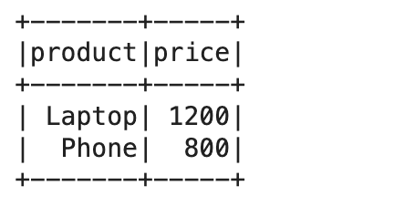
In this example, we will select specific columns and filter rows based on a condition. Assume we are working with a DataFrame containing order data.
from pyspark.sql import SparkSession
from pyspark.sql.functions import col

spark = SparkSession.builder.appName("SQLFunctions").getOrCreate()

data = [
    ("1001", "Laptop", 2, 1200, "2023-01-15"),
    ("1002", "Phone", 1, 800, "2023-01-20"),
    ("1003", "Tablet", 5, 300, "2023-02-01")
]

columns = ["order_id", "product", "quantity", "price", "order_date"]
orders_df = spark.createDataFrame(data, schema=columns)

selected_df = orders_df.select("product", "price")

filtered_df = selected_df.filter(col("price") > 500)

filtered_df.show()
Here is the output.
Transforming Data with SQL Functions
You can perform different transformations on data with Spark SQL functions like filter(), agg() (which stands for aggregate), groupBy(), and, finally, withColumn(). These functions:
- Allow conditions for more advanced row-based filtering
- Ability to add columns on top of other ones.
- Provide powerful aggregation operations (folder sum avg values).
- Implement Filters and add Sorting to display data in the order you want.
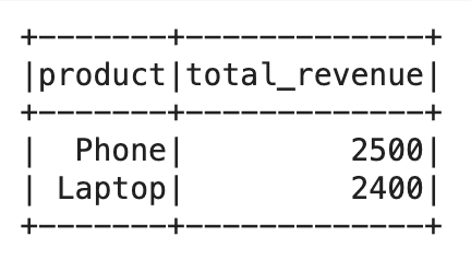
Let me illustrate this with an example using these combined operations to transform a dataset.
Scenario
You have a dataset containing the orders on products, and you need to —
- Select orders where the price > 500
- Create a new column ( total_cost = quantity * price)
- Group the orders at a product level and determine how much total revenue has come for each product.
- Products — Total Revenue (Dec)
Here is the code.
from pyspark.sql import SparkSession
from pyspark.sql.functions import col, sum, expr, desc
spark = SparkSession.builder.appName("TransformingData").getOrCreate()

data = [
    ("1001", "Laptop", 2, 1200, "2023-01-15"),
    ("1002", "Phone", 1, 800, "2023-01-20"),
    ("1003", "Tablet", 5, 300, "2023-02-01"),
    ("1004", "Monitor", 3, 150, "2023-02-10"),
    ("1005", "Phone", 2, 850, "2023-02-12")
]
columns = ["order_id", "product", "quantity", "price", "order_date"]
orders_df = spark.createDataFrame(data, schema=columns)

filtered_df = orders_df.filter(col("price") > 500)

transformed_df = filtered_df.withColumn("total_cost", col("quantity") * col("price"))

grouped_df = transformed_df.groupBy("product").agg(sum("total_cost").alias("total_revenue"))

final_df = grouped_df.orderBy(desc("total_revenue"))

final_df.show()
Here is the output.
Practical Examples
Practical examples of SQL functions in PySpark typically involve:
- Filtering rows based on specific conditions.
- Aggregating data, such as calculating totals or averages.
- Joining multiple DataFrames for enhanced analysis.
- Creating new columns based on existing data.
Let’s explore two practical examples of data transformations and analyses using SQL functions in PySpark.
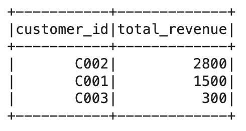
Customer Purchase Analysis
Imagine you are tasked with analyzing customer purchases at an online store. You need to calculate each customer's total revenue in a specific period and find the top five highest-spending customers.
from pyspark.sql import SparkSession
from pyspark.sql.functions import col, sum, expr, desc

spark = SparkSession.builder.appName("TransformingData").getOrCreate()

data = [
    ("1001", "Laptop", 2, 1200, "2023-01-15"),
    ("1002", "Phone", 1, 800, "2023-01-20"),
    ("1003", "Tablet", 5, 300, "2023-02-01"),
    ("1004", "Monitor", 3, 150, "2023-02-10"),
    ("1005", "Phone", 2, 850, "2023-02-12")
]

columns = ["order_id", "product", "quantity", "price", "order_date"]
orders_df = spark.createDataFrame(data, schema=columns)

filtered_df = orders_df.filter(col("price") > 500)

transformed_df = filtered_df.withColumn("total_cost", col("quantity") * col("price"))

grouped_df = transformed_df.groupBy("product").agg(sum("total_cost").alias("total_revenue"))

final_df = grouped_df.orderBy(desc("total_revenue"))

final_df.show()
Here is the output.
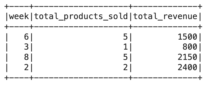
Weekly Sales Summary
Let’s say you’re asked to generate a weekly summary of total sales for a retail store. You need to calculate the total number of products sold each week and the total revenue generated.
Here is the code to do that;
from pyspark.sql import SparkSession
from pyspark.sql.functions import col, weekofyear, sum

spark = SparkSession.builder.appName("WeeklySalesSummary").getOrCreate()

sales_data = [
    ("Laptop", 2, 1200, "2023-01-15"),
    ("Phone", 1, 800, "2023-01-18"),
    ("Tablet", 5, 300, "2023-02-10"),
    ("Monitor", 3, 150, "2023-02-25"),
    ("Phone", 2, 850, "2023-02-26")
]

columns = ["product", "quantity", "price", "sale_date"]
sales_df = spark.createDataFrame(sales_data, schema=columns)

sales_df = sales_df.withColumn("total_cost", col("quantity") * col("price"))

sales_df = sales_df.withColumn("week", weekofyear(col("sale_date")))

weekly_summary_df = sales_df.groupBy("week").agg(
    sum("quantity").alias("total_products_sold"),
    sum("total_cost").alias("total_revenue")
)

weekly_summary_df.show()
Here is the output.
Customer Purchase Analysis: SQL functions like groupBy(), agg(), and orderBy() make it easy to compute totals and rankings.
Weekly Sales Summary: Date functions like weekofyear() and aggregation help generate meaningful time-based insights.
Performance Considerations

Let’s look at some techniques for performance considerations.
Optimization Techniques
Optimization in PySpark involves both improving the execution speed and reducing resource usage. Some essential techniques to optimize your PySpark jobs include:
- Partitioning: Dividing large datasets into smaller, manageable chunks for parallel processing.
- Caching and Persisting: Storing DataFrames in memory to avoid recomputation.
- Using Efficient Data Formats: Leveraging data formats like Parquet for faster read/write operations.
Handling Large Datasets
PySpark shines at being able to work with data that is larger than what traditional SQL tools could effectively handle. Here are a few tips for handling huge datasets in PySpark —
- Partitioning: PySpark attempts to distribute data across multiple partitions. However, you must correctly control the number of partitions to achieve high performance.
- Broadcast Joins: When one of the datasets is small but the other is huge, this PySpark broadcast join ensures that the large data is not shuffled no matter what happens.
- Persistence and Caching: If the same DataFrame is used several times in different transformations for any logic, it will benefit from caching since it is a very time-consuming operation.
Comparison with Traditional SQL
PySpark SQL is a highly scalable, distributed query engine suitable for big data applications. However, comparing it with traditional SQL approaches reveals significant differences, especially when handling large-scale datasets.
Key Differences
1. Distributed Computing: As we all know, traditional RBDMS processes data on a single machine (or, in other words, a clustered configuration for some advanced databases), while PySpark uses a distributed computing model across the cluster of nodes. This allows PySpark to process significantly massive data and execute high computational complexity queries in less time.
2. Fault Tolerance: ySpark SQL achieves this using resilient distributed datasets (RDDs) built into Apache Spark. The system will not lose any data because even if a piece was processing on some node that suddenly failed, the failed node could be detected and restarted or just send that chunk of bytes from “head” to another working replica for it to process. Although traditional SQL databases sometimes provide redundancy, they often rely on backups or, even worse, mirroring for recovery.
3. In-Memory Computation: The ability to use in-memory computation, such as iterative algorithms or repeated access to data, which Hadoop does not support. Traditional SQL engines typically have disk-based computation, which may be slower than in-memory processing, and incredibly complex analytical queries.
4. Data Size: Traditional SQL easily copes with small to medium datasets, but it needs an environment to handle large DB sizes. PySpark SQL, however, is built to effortlessly handle such massive data.
Advanced SQL Functions in PySpark
The advanced SQL functions of PySpark provide extensive support for complex data transformations and analyses, including windowed, user-defined functions (UDFs). These can rank, aggregate, and compute in smaller partitions according to where your data resides or provide custom operations for specific business requirements.
Window Functions
PySpark Window Functions calculates the subset of rows or windows based on special expressions defined as partitions based on specific column values.
These are great for ranking, cumulative totals, or calculating movements over an entire series. Window functions are not like regular aggregate functions because if you use windows, no rows collapse, and every individual row with its calculated values still shows up.
Use Case: Email Activity Ranking
Activity Rank
Last Updated: July 2021
Find the email activity rank for each user. Email activity rank is defined by the total number of emails sent. The user with the highest number of emails sent will have a rank of 1, and so on. Output the user, total emails, and their activity rank.
• Order records first by the total emails in descending order. • Then, sort users with the same number of emails in alphabetical order by their username. • In your rankings, return a unique value (i.e., a unique rank) even if multiple users have the same number of emails.
Here is the question we will use to explain window questions: https://platform.stratascratch.com/coding/10351-activity-rank
Here’s how we approach this:
1. Group by user: First, we group the messages by the sender (from_user) and count the number of emails each sends.
2. RANK USERS: We rank users by the total number of emails they have sent, and in case of a tie, we sort by usernames.
3. Order the result: Finally, we order by the total count of emails descending and then userName when there is a tie.
Here is the code.
import pyspark.sql.functions as F
from pyspark.sql.window import Window

result = google_gmail_emails.groupby('from_user').agg(F.count('*').alias('total_emails'))
result = result.withColumn('rank', F.row_number().over(Window.orderBy(F.desc('total_emails'), 'from_user')))
result = result.orderBy(F.desc('total_emails'), 'from_user')

result.toPandas()
Here is the output.
| from_user | total_emails | rank |
|---|---|---|
| 32ded68d89443e808 | 19 | 1 |
| ef5fe98c6b9f313075 | 19 | 2 |
| 5b8754928306a18b68 | 18 | 3 |
| 55e60cfcc9dc49c17e | 16 | 4 |
| 91f59516cb9dee1e88 | 16 | 5 |
| 6edf0be4b2267df1fa | 15 | 6 |
| 7cfe354d9a64bf8173 | 15 | 7 |
| cbc4bd40cd1687754 | 15 | 8 |
| e0e0defbb9ec47f6f7 | 15 | 9 |
| 8bba390b53976da0cd | 14 | 10 |
| a84065b7933ad01019 | 14 | 11 |
| e22d2eabc2d4c19688 | 13 | 12 |
| 850badf89ed8f06854 | 12 | 13 |
| aa0bd72b729fab6e9e | 12 | 14 |
| 2813e59cf6c1ff698e | 11 | 15 |
| 5dc768b2f067c56f77 | 11 | 16 |
| 5eff3a5bfc0687351e | 11 | 17 |
| 75d295377a46f83236 | 11 | 18 |
| 157e3e9278e32aba3e | 10 | 19 |
| d63386c884aeb9f71d | 10 | 20 |
| 406539987dd9b679c0 | 9 | 21 |
| 6b503743a13d778200 | 9 | 22 |
| 114bafadff2d882864 | 8 | 23 |
| 47be2887786891367e | 6 | 24 |
| e6088004caf0c8cc51 | 6 | 25 |
This method ensures that even users with the same number of emails will receive a unique rank based on their usernames.
What is a UDF in PySpark?
PySpark User Defined Function (UDF) is a feature that is available to solve such problems. Although PySpark contains many built-in functions for data transformations, UDFs allow you to define your transformation logic when standard functions are insufficient. Override a standard function definition.
- When to Use UDFs: You can write UDFs for those things you do on your rows in a customized way.
- Performance Considerations: UDFs are more computationally expensive than the built-in functions, but they can be partially compiled in Spark. So, these should be used only when the built-in functions do not satisfy.
Categorizing Users Based on Email Activity
Let's apply a UDF to categorize users based on their total email activity. We will:
1. Group by the users who sent emails.
2. Count how many emails each user has sent.
3. Use a UDF to categorize each user based on their activity:
- Power User: Sent more than 10 emails.
- Moderate User: Sent between 5 and 10 emails.
- Low Activity: Sent fewer than 5 emails.
Step-by-Step Implementation:
We'll use a predefined dataset (google_gmail_emails) that records user email exchanges.
That explains what we will do,
1. Group by and Count: We group the google_gmail_emails data frame with from_user, which is the count of emails each user sends.
2. Define UDF: The UDF categorize_user_activity is a function that receives the number of emails (total) as input and gives you what category the user should be in based on predefined thresholds(Power User, Moderate User, Low Activity).
3. Register UDF: We register the UDF using PySpark's function, simply presented using the unspecified return type StringType().
4. UDF Application: We apply the UDF to the dut_total sort column and create a new user_category, where each row is transformed to fit its respective user category.
5. Display Results: Lastly, display the DataFrame with from_user, total_emails and user_category.
Here is the code.
import pyspark.sql.functions as F
from pyspark.sql.types import StringType
from pyspark.sql import SparkSession

spark = SparkSession.builder.appName("EmailActivityClassification").getOrCreate()

data = [
    ('user1', 'user2', 1),
    ('user1', 'user3', 2),
    ('user1', 'user4', 3),
    ('user2', 'user3', 4),
    ('user3', 'user1', 5),
    ('user3', 'user2', 6),
    ('user3', 'user4', 7),
    ('user3', 'user5', 8),
    ('user2', 'user1', 9),
    ('user2', 'user4', 10),
    ('user4', 'user1', 11),
    ('user4', 'user3', 12)
]

columns = ['from_user', 'to_user', 'email_id']

google_gmail_emails = spark.createDataFrame(data, columns)

email_counts = google_gmail_emails.groupBy('from_user').agg(F.count('*').alias('total_emails'))

def categorize_user_activity(total_emails):
    if total_emails > 10:
        return "Power User"
    elif 5 <= total_emails <= 10:
        return "Moderate User"
    else:
        return "Low Activity"

categorize_udf = F.udf(categorize_user_activity, StringType())

email_counts_with_category = email_counts.withColumn("user_category", categorize_udf(F.col("total_emails")))

email_counts_with_category.show()
Here is the output.
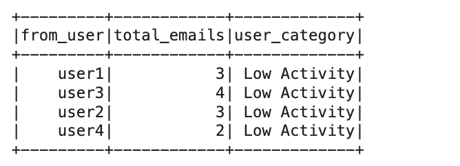
This example demonstrates using a UDF in PySpark to apply custom logic to classify users based on their email activity. While PySpark has many built-in functions, UDFs are helpful when implementing custom logic not covered by existing functions.
Common Pitfalls and Best Practices
PySpark SQL is a great tool for working with data, but you should learn some performance tricks to maximize its benefits.
- Non-optimized Joins: Joins between two large datasets are expensive and affect job running time. For relatively small datasets, leverage broadcast joins to avoid expensive shuffles.
- Data Formats: CSV files; processing is slow. It also uses the Parquet / ORC format for better compression and fast read/write operations.
- Inaccurate Partitioning: Adding and decreasing the number of partitions will not work well. One practical advice is to change partitioning according to data size and the resources of a cluster.
- Excessive Use of Collect (): Fetching full data to a single machine (driver) can exhaust its memory. Use. Use show() or take() for minor sample inspections.
To apply what you have learned, read PySpark Interview Questions, which includes PySpark questions.
Conclusion
In this article, we have discovered PySpark SQL Functions and how they can be used using real-life datasets from actual interview questions. We also found high-level functions, common pitfalls to avoid, and performance considerations.
To solidify your knowledge, make sure to do regular practices. On the StrataScratch platform, you can see datasets where you can apply this knowledge or solve interview questions with pyspark.
Share