Machine Learning Algorithms Explained: Clustering

In this article, we are going to learn how different machine learning clustering algorithms try to learn the pattern of the data.

Let’s imagine that on a Saturday night, our friends invite us to a concert by a band that we have never heard of. When they play their music, you notice that there are no lyrics at all in their song. Although you just listened to their music for the very first time, you might guess that their music is one of the instrumental genres.

Your ability to be able to classify music genres as you listen to them for the very first time is one of the examples of clustering in real life. Clustering is one of the unsupervised learning methods in the machine learning paradigm. The main goal of machine learning clustering algorithms is to assign an instance or unseen data point to a particular group without the need to assign a ground-truth label in advance.

There are a lot of use cases in real life where clustering method will be beneficial, such as:

• Customer and market grouping
• Image segmentation
• Social media analysis
• Search engine result grouping
• Anomaly detection

To understand the high-level concept behind machine learning clustering, let’s take a look at the following data points:

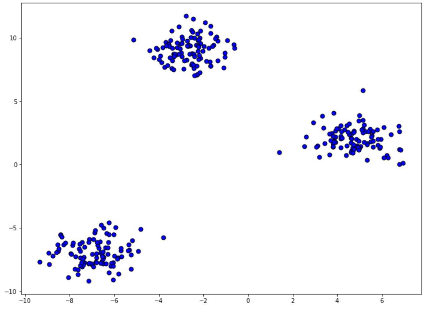
At a first glance, the scattered data points above are just data points, each with its own x-coordinate and y-coordinate. There is no label or ground truth available for each data point. Now, the task of our machine learning algorithm is to try to learn the pattern of these scattered data points by itself and then assign each of the data points to a particular group.

The clustering result of the scattered data points above might look something like this:

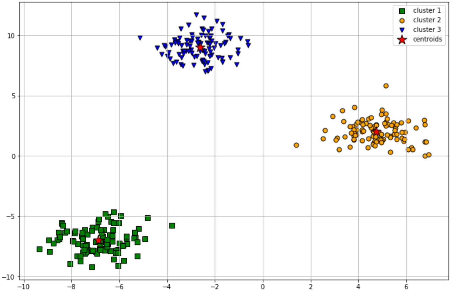
As you can see in the visualization above, the data points that are considered ‘similar’ by our machine learning model are grouped together into one cluster. Overall, our machine learning model did a great job in two things:

1. Determining the necessary number of clusters
2. Assigning each data point to the most likely cluster

Now the question that we might ask is, how does our machine learning model determine the optimum number of clusters? How does our machine learning model assign each data point to the most suitable clusters?

Different machine learning algorithms have their own way and concept of how to come up with the optimum number of clusters as well as how they assign each data point to the appropriate cluster. In this article, we’re going to learn how different machine learning clustering algorithms try to learn the pattern of the data to come up with the things mentioned above.

So, let’s start with different types of machine learning clustering algorithms.

Types of Machine Learning Clustering Algorithms

There are many types of machine learning clustering algorithms, but in this article we’re going to cover four of the most commonly used clustering algorithms.

Centroid-Based Clustering

Centroid-based machine learning clustering is a method where the algorithm needs to first randomly initialize a certain amount of centroids that should be defined in advance. This algorithm will then use an iterative approach to find the optimum position for each centroid such that the distance between data points and the centroid is minimized.

The most crucial part of this method is defining the number of centroids that should be initialized in advance before the iterative step takes place. In the next section, we’re going to take a look at an approach that utilizes centroid-based clustering. There we will learn how we can determine the optimum number of clusters for our use case.

Distribution-Based Clustering

Distribution-based clustering is a clustering method that uses probability from a particular distribution to group data points into clusters instead of using similarity or distance as the metrics.

Specifically, it groups data points based on each data point’s likelihood of belonging to a specific probability distribution, which commonly would be the Gaussian distribution. However, you can choose different probability distributions as well, such as Binomial distribution.

Density-Based Clustering

As the name suggests, density-based clustering is a clustering algorithm that works by identifying and grouping data points that are located in the same high-density region together.

This clustering method can cluster data points together in an arbitrary shape, as long as the data points are located close to each other in a dense region.

Hierarchical-Based Clustering

Hierarchical-based clustering is a machine learning clustering algorithm that groups data points into clusters by looking at the distance between each data point and its neighborhood. With this method, each data point is connected to its neighbors depending on their distance and then the data points that have minimal distance among them would be clustered into one group.

To achieve the purpose above, hierarchical-based clustering uses either one of two different approaches:

• Agglomerative approach: This approach starts by taking a single data point as a single cluster, and merges all of the data points such that in the end, we end up with a single cluster. We’re going to learn more about how this works in the next section.
• Divisive approach: This approach is the opposite of the agglomerative approach. The idea behind this approach is that we assume that initially, all of the data points belong to one large cluster. Next, this approach tries to split this large cluster into smaller clusters based on specific distance thresholds or until we reach a point where further data splitting is no longer possible.
  

We can normally visualize a hierarchical-based approach with the dendrogram visualization that you will also see in more detail in the next section. This method looks similar to the tree-based machine learning method and if you would like to learn more about the tree-based machine learning method, you can read it here: “Decision Tree and Random Forest Algorithm Explained”.

Now that we know about different kinds of clustering methods, let’s take a look at different types of machine learning clustering algorithms that utilize each of the approaches mentioned above. Let’s start with k-means clustering.

k-Means Clustering in Machine Learning

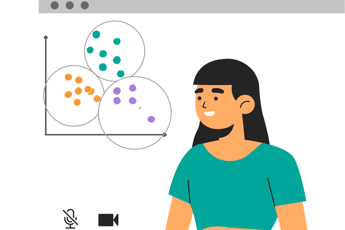
k-means clustering in machine learn is one of the algorithms that utilize the centroid-based clustering approach. Among several machine learning algorithms commonly used for clustering purposes, k-means clustering is arguably the most common one to be used. The reason for this is that of course, it normally performs reasonably well and also, the working concept of k-means clustering can be easily explained.

To understand how k-means clustering actually works, let’s imagine that we have scattered data points as follows:

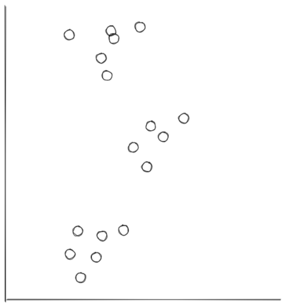
From our perspective, we know how the final clustering should look like: it should have three clusters that looks something like the following:

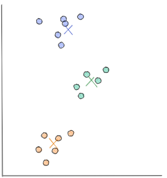
And the visualization above is exactly what we’re going to get after implementing the k-means clustering algorithm. Now the question is, how is the k-means clustering algorithm able to cluster our data points as shown in the visualization above?

Below is the step-by-step working process of k-means clustering in machine learning:

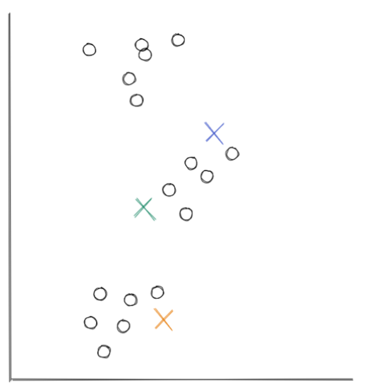
• The first step of centroid-based clustering is defining the number of clusters, and we need to define it in advance. Each centroid will act as the center of the cluster. As an example, let’s say that we initialize three centroids in the beginning, this means that we have three clusters formed in the end. The centroids that we initialized will then be placed randomly by this algorithm at the start, as you can see in the visualization below:

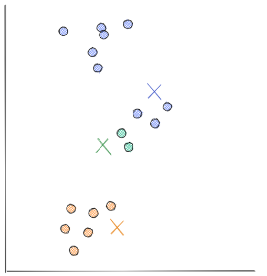
• After random initialization, now the similarity between each centroid and each data point is calculated. The measure of similarity usually used in centroid-based clustering is the distance, which can be calculated by using Euclidean distance. After calculating the distance, then each data point will be assigned to the nearest centroid, as you can see in the visualization below:

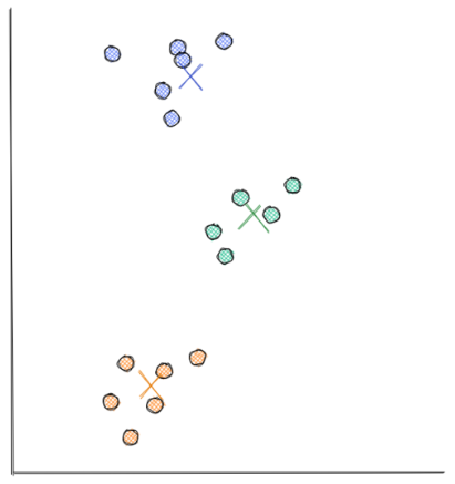
• In the third step, each centroid will move to the average point of data points assigned to it. As already mentioned in the previous section, centroid-based clustering utilizes an iterative approach to come to the optimal solution. This is the end of the first iteration.

• The second iteration follows the same step as the previous iteration. In this step, the similarity or the distance of the data points to the closest centroid that’s already moved to its new position is computed again. Then, same as the previous iteration, each data point will be assigned to the closest centroid.

• Next, each centroid moves to the average of data points assigned to it, as you can see in the visualization below. This step is the end of the second iteration, and the third iteration will follow the same procedure described in the previous steps. In our example case, the algorithm has reached the optimal solution at the end of the second iteration. This means that the position of each centroid will no longer move, even if we run this algorithm for many more iterations.

Choosing the Number of Centroids

The letter k in k-means clustering algorithm refers to the number of clusters. As already mentioned in the previous section, the important step of a centroid-based algorithm is to define the number of clusters in advance. The problem is that we don’t normally have any prior information about the optimal number of clusters that we should initialize.

If we initialize too few centroids, then the clustering result would not lead to a good result. Meanwhile, if we initialize too many centroids, then there would be an overfitting problem such that the clustering result would be meaningless.

However, there is an approach commonly used in the k-means clustering algorithm to come up with the optimal number of centroids that need to be initialized, which is called the elbow method. To use this method, we initialize a different number of clusters and then track the sum of in-group errors.

The in-group error or also commonly called within-group error measures how well is each centroid in approximating our data. More centroids mean lesser in-group error, but in k-means clustering, a lower value of in-group error doesn’t mean that the clustering result becomes better. A very low value of in-group error means that the clustering result is basically meaningless, as you can imagine that one centroid represents only one data point. What we want instead is to find that number of clusters that results in an in-group error that’s low ‘enough’, but not too low.

With the so-called elbow method, we will normally get the following visualization from the number of clusters vs the in-group error:

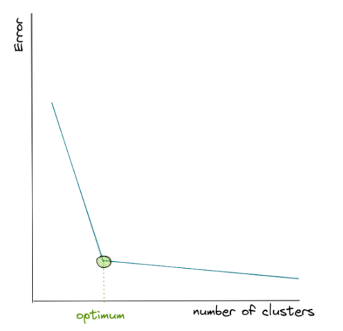
The in-group error keeps decreasing as we increase the number of centroids. However, after a certain number of clusters, the error decreases at a slower rate, which gives us an elbow-shaped visualization. The optimum number of clusters will be the one where the elbow shape is formed, as you can see with the green circle above.

Implementation of k-Means Clustering

Let’s now implement k-means clustering in Python. In this example, we’re going to use the Scikit-learn library to do so, specifically with the KMeans instance from sklearn.cluster. But first, let’s generate the dataset first.

import matplotlib.pyplot as plt
from sklearn.datasets import make_blobs

# create dataset
X, y = make_blobs(
   n_samples=300, n_features=2,
   centers=3, cluster_std=1,
   shuffle=True, random_state=42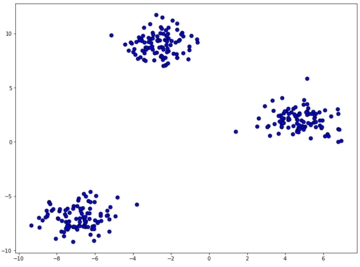

As you can see from the visualization above, our dataset consists of 300 data points, and from the location of our data points, we would expect that the k-means clustering method will be able to form three clusters. However, if you remember, we need to define the number of centroids in advance. In our case, we know that it should be 3, but in most real-life scenarios, we don’t know how many centroids we should define.

To solve this, we’re going to use the Elbow method explained in the previous section. So let’s find out if this method will give us 3 as the optimum number of centroids.

from sklearn.cluster import KMeans
from matplotlib import pyplot as plt

errors = []
for k in range(1, 10):
    kmeans = KMeans(n_clusters=k)
    kmeans.fit(X)
    errors.append(kmeans.inertia_)

fig = plt.figure(figsize=(12, 9))
plt.plot(range(1, 10), errors)
plt.grid(True)
plt.xlabel('Error', fontsize=18)
plt.ylabel('No. of clusters', fontsize=16)
plt.title('Elbow curve',fontsize=18)

With the elbow method, we can clearly see that the optimum number of clusters would be 3. So, let’s initialize and train a new k-means clustering model, and then plot the clustering result as well as the location of each centroid.

# Initialize and train k-means model
km = KMeans(n_clusters=3)
y_kmeans = km.fit_predict(X)

# plot the clusters and centroids
plt.figure(figsize=(12,8))
plt.scatter(
    X[y_kmeans == 0, 0], X[y_kmeans == 0, 1],
    s=50, c='green',
    marker='s', edgecolor='black',
    label='cluster 1'
)

plt.scatter(
    X[y_kmeans == 1, 0], X[y_kmeans == 1, 1],
    s=50, c='orange',
    marker='o', edgecolor='black',
    label='cluster 2'
)

plt.scatter(
    X[y_kmeans == 2, 0], X[y_kmeans == 2, 1],
    s=50, c='blue',
    marker='v', edgecolor='black',
    label='cluster 3'
)

plt.scatter(
    km.cluster_centers_[:, 0], km.cluster_centers_[:, 1],
    s=250, marker='*',
    c='red', edgecolor='black',
    label='centroids'
)
plt.legend(scatterpoints=1)
plt.grid()
plt.show()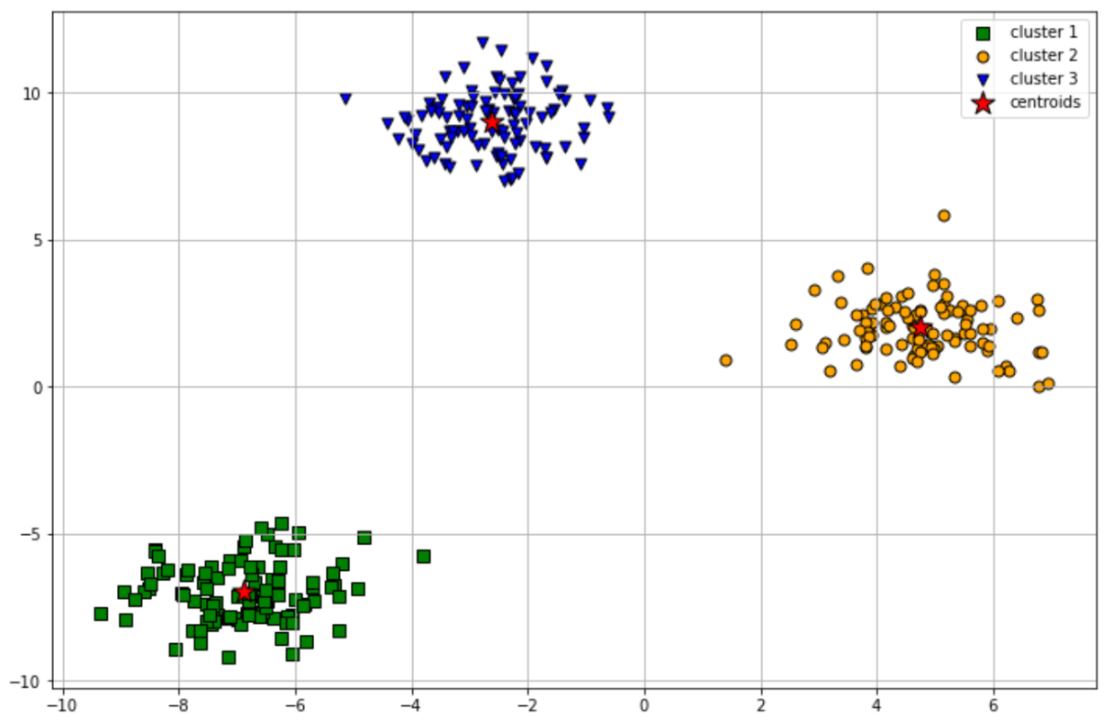

As you can see from the visualization above, our k-means clustering algorithm managed to group our data points into 3 clusters perfectly. However, the k-means clustering algorithm has a couple of drawbacks that make this algorithm wouldn’t be the right algorithm to use in a certain use case. We will find out more about this in the next section.

Gaussian Mixture Model for Clustering in Machine Learning

As mentioned previously, there are certain drawbacks of using the k-means clustering algorithm. K-means clustering performs best when our dataset has a circular shape, as you can see from the previous example.

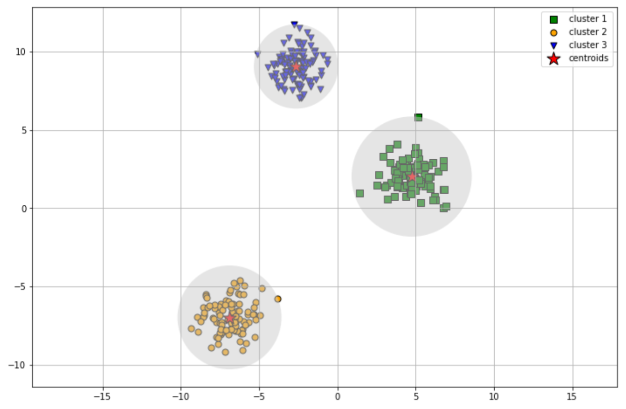
If we have data points that can’t be clustered with circular shape, then the k-means clustering algorithm will perform poorly, as you can see in the following visualization:

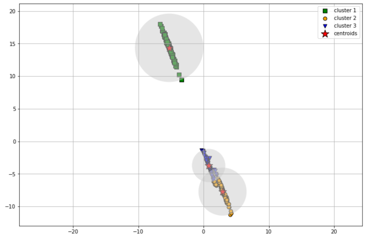
As you can see, the k-means clustering algorithm couldn’t cluster our data points properly as some of the data points are wrongly clustered. Also, k-means clustering results in a hard classification of clusters, which means that each data point will get a result in which cluster it has been assigned to.

Gaussian Mixture Model or GMM is a probabilistic-based clustering method that alleviates the problem with k-means clustering above. GMM assumes that each data point comes from a mixture of several Gaussian distributions with unknown parameters (mean and standard deviation).

Below is the step for how data points can be generated with GMM:

• First, the number of Gaussian distributions needs to be defined, let’s say the number of Gaussian distributions is k and we will call this the number of clusters. The parameters (mean and standard deviation) of each Gaussian distribution are normally assigned randomly
• One random cluster is picked from a possible k Gaussian distribution for each data point with a certain probability value of choosing i th cluster defined by the cluster’s weight.
• Finally, the location of each data point is sampled randomly from the chosen Gaussian distribution in the ith cluster with a certain mean and covariance matrix.
• The parameters (mean, standard deviation, and weight) of each cluster will be updated iteratively based on data points assigned to it.

The main goal of GNN is to find in which Gaussian distribution a data point is most likely to be generated. To achieve this, GMM uses an iterative approach in order to optimize the Gaussian distributions’ parameters that are normally initialized randomly in the beginning. This involves two steps:

• First, GMM will assign each data point to a cluster (Gaussian distribution) similar to assigning data points to a centroid in the k-means algorithm. This step is also normally called the expectation step. This step tries to answer the following: does the data point look likely to be generated by the ith cluster?
• Then, the parameters of each cluster will be updated according to the data points assigned to it. This step is also normally called the maximization step.

Choosing the Number of Clusters

The similar concept between GMM and k-means clustering is that we need to define the number of clusters in advance. Specifically in GMM, we need to define the number of distributions that we should initialize, whereas in k-means clustering we need to define the centroids.

With k-means, we know we can use the elbow method to determine the optimal number of centroids. But how about in GMM? The main approach in GMM is that we need to initialize a certain number of clusters such that the so-called theoretical information criterion is minimized. Examples of theoretical information criteria would be Bayesian information criterion (BIC) and Akaike information criterion (AIC).

Below are the equations for BIC and AIC:

where:

m: data points

p: parameters that need to be optimized by GMM

L: the likelihood function

By plotting the AIC or BIC against the number of distributions, we will normally get similar visualization as in the elbow method as follows:

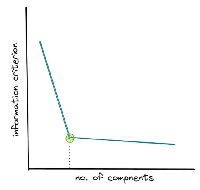
The information criterion keeps decreasing as we increase the number of distributions. However, same as the elbow method in k-means clustering, we want to select the number of distributions where the elbow shape is formed, as you can see in the green dot above.

Implementation of Gaussian Mixture Model

Now that we know at a high level how GMM works, let’s implement it with the help of Python. Same as before, we’re going to use the scikit-learn library to do so. For this GMM example, we’re going to use the stretched dataset as visualized above.

But before moving further, the first step that we need to do is to define the number of Gaussian distributions. Same as k-means clustering algorithm, normally we don’t know how many distributions we should define in advance. However intuitively, we know that the optimal number of distributions would be 3. Let’s find out about this by plotting the AIC and BIC criterion vs the number of distributions.

from sklearn.mixture import GaussianMixture
import numpy as np

rng = np.random.RandomState(52)
X_stretched = np.dot(X, rng.randn(2, 2))

n_components = np.arange(1, 10)

gm = [GaussianMixture(n, covariance_type='diag', random_state=0).fit(X_stretched) for n in n_components]

plt.figure(figsize=(12,8))
plt.plot(n_components, [m.bic(X_stretched) for m in gm], label='BIC')
plt.plot(n_components, [m.aic(X_stretched) for m in gm], label='AIC')
plt.legend(loc='best')
plt.xlabel('n_components', fontsize=18);
plt.ylabel('information criterion', fontsize=16);
plt.grid(True)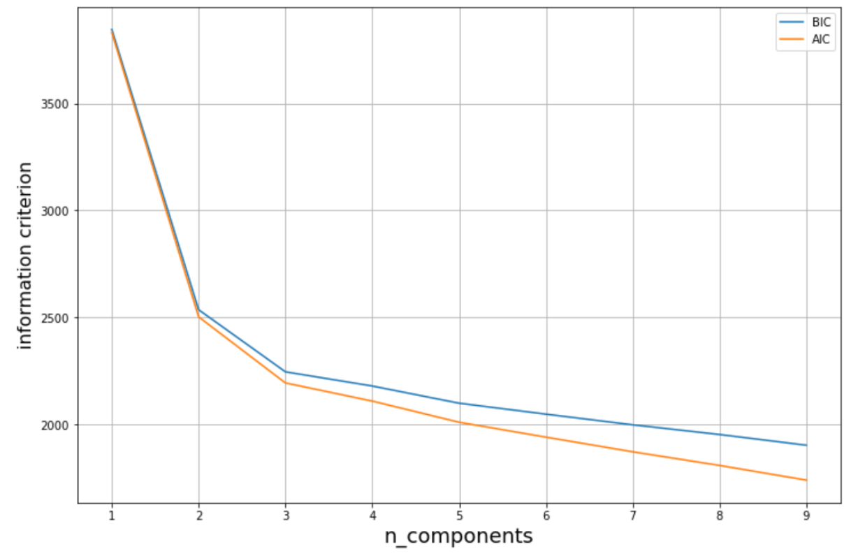

As you can see in the visualization above, the elbow shape is formed when the number of distributions is 3. Hence, it is safe for us to assume that the optimal number of distributions for our use case is 3.

Let’s initialize and train the GMM model on our data points with 3 clusters. After that, we can visualize the clustering result

from matplotlib.patches import Ellipse

def draw_ellipse(position, covariance, ax=None, **kwargs):
    ax = ax or plt.gca()
    
    if covariance.shape == (2, 2):
        U, s, Vt = np.linalg.svd(covariance)
        angle = np.degrees(np.arctan2(U[1, 0], U[0, 0]))
        width, height = 2 * np.sqrt(s)
    else:
        angle = 0
        width, height = 2 * np.sqrt(covariance)
    
    for nsig in range(1, 4):
        ax.add_patch(Ellipse(position, nsig * width, nsig * height,
                             angle, **kwargs))

def plot_scatter(X, labels, target, color, marker_shape, legend):
        
    plt.scatter(
    X[labels == target, 0], X[labels == target, 1],
    s=50, c=color,
    marker=marker_shape, edgecolor='black',
    label=legend
    )
    
def plot_gmm(gmm, X, label=True, ax=None):
    plt.figure(figsize=(12,8))
    ax = ax or plt.gca()
    labels = gmm.fit(X).predict(X)
    if label:

        plot_scatter(X, labels, 0, 'green', 's', 'cluster_1')
        plot_scatter(X, labels, 1, 'orange', 'o','cluster_2')
        plot_scatter(X, labels, 2, 'blue', 'v','cluster_3')

    ax.axis('equal')
    plt.grid(True)
    
    
    w_factor = 0.2 / gmm.weights_.max()
    for pos, covar, w in zip(gmm.means_, gmm.covariances_, gmm.weights_):
        draw_ellipse(pos, covar, alpha=w * w_factor)

gmm = GaussianMixture(n_components=3, covariance_type='full', random_state=42)
plot_gmm(gmm, X_stretched)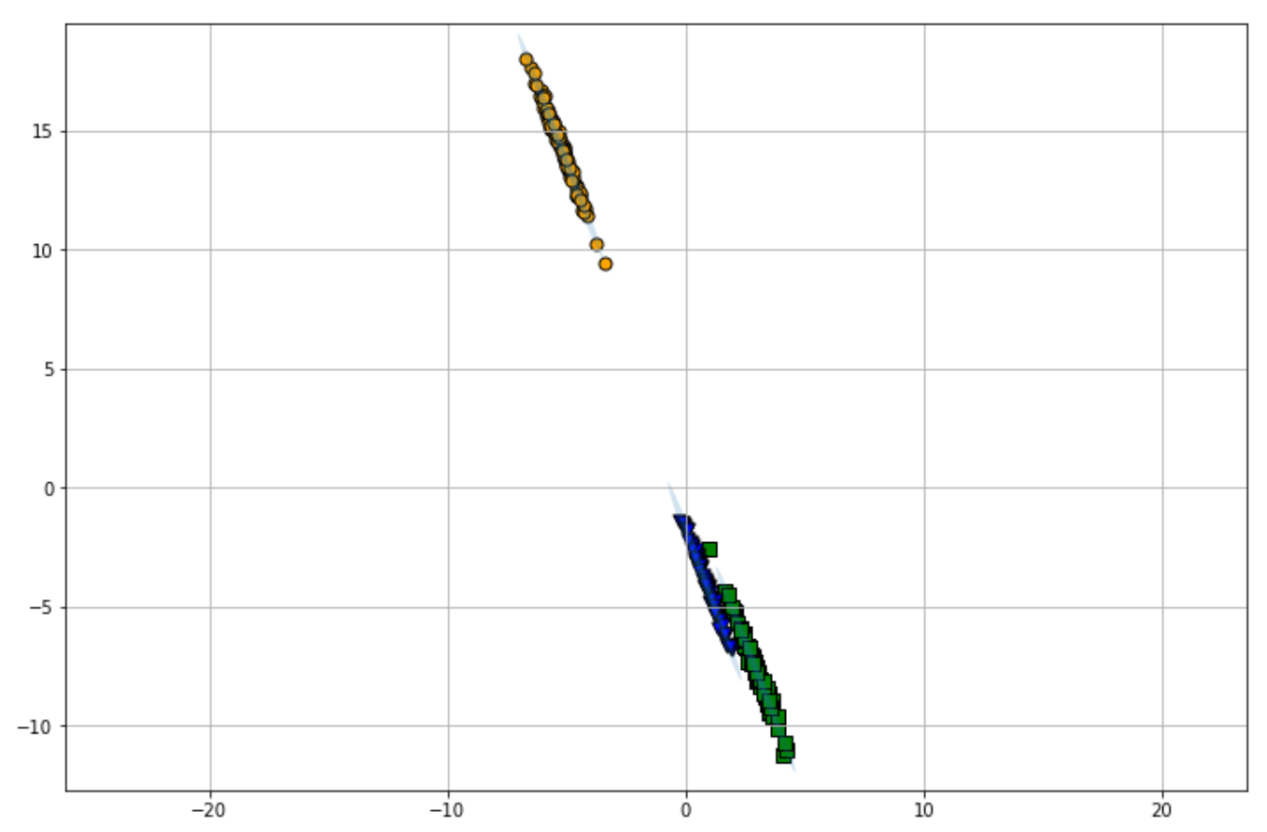

As you can see, GMM gives us flexibility in terms of the shape of the clusters. Instead of a circular shape cluster, GMM can also capture an ellipsis shape cluster, hence the better clustering result for our use case above.

Agglomerative Clustering in Machine Learning

The agglomerative clustering algorithm in machine learning is a hierarchical-based clustering method that we can also use to cluster our data points. One advantage of using agglomerative clustering instead of the previous two algorithms is that we don’t really need to initialize a specific number of clusters in advance if we don’t want to.

However, although we don’t really need to initialize a specific number of clusters in advance, the clustering result would be potentially better if we specify the optimal number of clusters in advance. With agglomerative clustering, there is a certain way to find out the optimal number of clusters, which we will discuss in the next section.

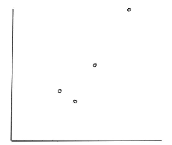
In a nutshell, an agglomerative algorithm works by first assigning each data point as a cluster. Let’s say we have 4 data points, then in the beginning we would have 4 clusters. Next, the algorithm merges the data points iteratively such that in the end, we end up with one single big cluster containing all of the data points.

To understand more how the agglomerative algorithm works, let’s say that in the beginning we have data with four data points, as you can see below:

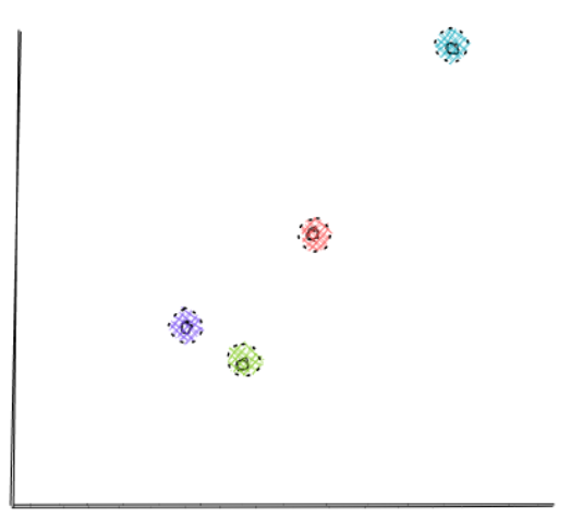
In the first iteration, each data point will be assigned as a single cluster. If we have N data points, then we will have N clusters at this point.

In the next iteration, the two closest data points will be merged together, such that after this iteration, we have N-1 clusters.

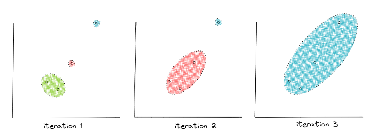
The steps above will be repeated iteratively until it forms into a single cluster. Once they form into a single cluster, then the merging history in each iteration can be visualized with the dendrogram.

Now the question is, how does this merging of points work? How does the algorithm choose which data points will be merged in each iteration? The distance between two data points across different clusters is normally used, and there are two common metrics that the agglomerative approach uses to calculate this distance:

• Single linkage: The distance is calculated from the closest data points in-between clusters
• Complete linkage: The distance is calculated from the farthest data points in-between clusters
• Centroid linkage: The distance is calculated from the centroid of each cluster.
• Ward linkage: The distance is calculated such that the variance of the clusters being merged is minimized

Choosing the Number of Clusters

As mentioned previously, although it’s not mandatory, the clustering result of the agglomerative clustering is often better when we decide the number of clusters in advance. Now the question is, how do we know the optimal number of clusters?

Previously we have learned how agglomerative clustering works in a nutshell. In the end, we can visualize the merging history in each iteration with the so-called dendrogram. The dendrogram visualization will help us to determine the optimal number of clusters for our use case.

In general, the visualization of a dendrogram would look something like this:

The y-axis in the above visualization represents the distance and the x-axis represents our data points. To determine the optimal number of clusters from the visualization above, here is the common step-by-step procedure:

• Draw a horizontal line that will act as a cut-off point on the tallest vertical line that doesn’t intersect with any other cluster.
• The number of vertical lines that intersect the horizontal line would be the optimal number of clusters. In the following visualization, the optimal number of clusters would be 3

Of course, there is a possibility that we will get a different number of clusters if we choose different cut-off points (distance). This is why we need to adjust this algorithm according to our needs and knowledge about the data.

Implementation of Agglomerative Algorithm

Now that we know how agglomerative approach works, let’s try to implement this algorithm with Python. We will use the same dataset that we used in the previous two machine learning clustering algorithms.

First, let’s visualize the dendrogram of the merging history for our use case in order to determine the optimal number of clusters.

import pandas as pd
import numpy as np
from matplotlib import pyplot as plt
from sklearn.cluster import AgglomerativeClustering
import scipy.cluster.hierarchy as sch

plt.figure(figsize=(12, 8))
dendrogram = sch.dendrogram(sch.linkage(X, method='ward'))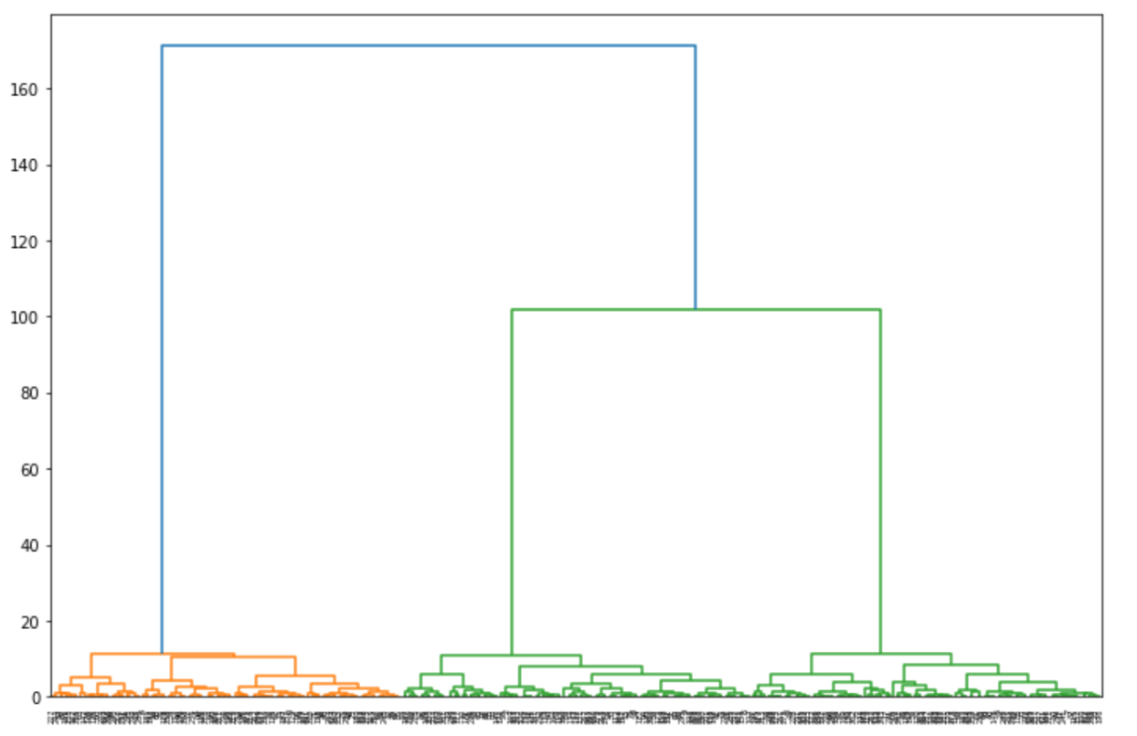

From the visualization above, let’s pick the cut-off point at 80. Then we can draw a horizontal line from there and find out that the optimal number of clusters would be 3.

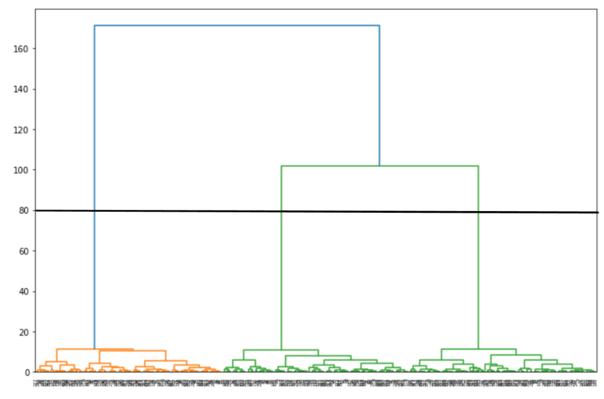
Now let’s instantiate our agglomerative model with 3 clusters and train it on our dataset. Next, we can visualize the clustering result.

def plot_scatter(X, labels, target, color, marker_shape, legend):
        
    plt.scatter(
    X[labels == target, 0], X[labels == target, 1],
    s=50, c=color,
    marker=marker_shape, edgecolor='black',
    label=legend
    )
    
def plot_agglo(agglo, X, label=True, ax=None):
    plt.figure(figsize=(12,8))
    ax = ax or plt.gca()
    labels = agglo.fit_predict(X)
    if label:
        
        plot_scatter(X, labels, 0, 'green', 's', 'cluster_1')
        plot_scatter(X, labels, 1, 'orange', 'o','cluster_2')
        plot_scatter(X, labels, 2, 'blue', 'v','cluster_3')

    ax.axis('equal')
    plt.grid(True)

agglo = AgglomerativeClustering(n_clusters=3, affinity='euclidean', linkage='ward')
plot_agglo(agglo, X)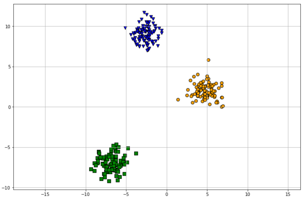

As mentioned before, one of the advantages of using the agglomerative ML clustering algorithm is that we don’t need to initialize a certain number of clusters in advance. What we can do instead is to define the threshold distance of the linkage. This means that if the distance between two clusters is above the threshold, then the agglomerative algorithm won’t merge the clusters.

To make it clearer, let’s do some examples in Python without defining a specific number of clusters. We’re going to specify two different distances: 60 and 140, and then let’s see the difference in the clustering result between these two.

agglo_dist_60 = AgglomerativeClustering(n_clusters=None, distance_threshold=60, affinity='euclidean', linkage='ward')
agglo_dist_140 = AgglomerativeClustering(n_clusters=None, distance_threshold=140, affinity='euclidean', linkage='ward')

plot_agglo(agglo_dist_60, X)
plot_agglo(agglo_dist_140, X)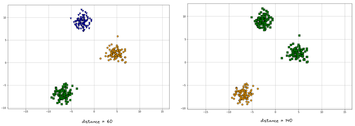

There is one apparent difference between the two visualizations above: on the left-hand side, we ended up having 3 clusters, while on the right-hand side we ended up having just 2. Indeed, the result from 3 clusters is better than 2, but the question is, why do we end up with a different number of clusters just by changing the distance threshold?

If you look at the dendrogram visualization above, if our cut-off point is 60 and we draw a horizontal line across the graph, then it will intersect 3 different vertical lines, which corresponds to our visualization result. Meanwhile, if our cut-off point is 140 and we draw the horizontal line, it will intersect only 2 vertical lines, which also corresponds to our visualization result on the right-hand side.

This is why the threshold distance can be considered as one of several hyperparameters that we should tune in order to get a better clustering result. Other hyperparameters that we can fine-tune are the type of linkage as well as the distance metrics.

As an example, ward linkage often performs best when we have a cluster with a spherical shape, while with a single linkage, although it might not be robust to the outlier, it performs well in a cluster with an arbitrary shape. Let’s imagine we have the following data points:

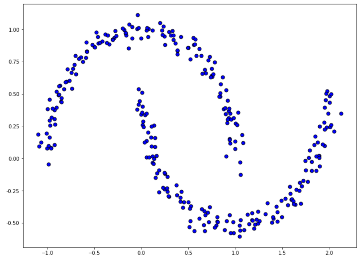
Now, if we implement agglomerative clustering with two different linkage methods, ward and single, we will end up with the following results:

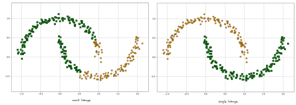
On the left-hand side, the clustering result is not optimal with ward linkage, as it’s generally not suited to find a cluster with arbitrary shape. Meanwhile on the right-hand side, the clustering result is much better when we use single linkage.

DBSCAN in Machine Learning

Density-based spatial clustering of applications with noise or DBSCAN is a density-based clustering method that calculates how dense the neighborhood of a data point is. In a nutshell, DBSCAN works similarly to the algorithms mentioned in the previous section. First, it will measure the similarity between data points, and group similar data points into one cluster. One of the best advantages of the DBSCAN clustering algorithm is that it is able to find a cluster with an arbitrary shape.

Let’s imagine that we have data points that look like the moon datasets visualized above. If we’re using k-means clustering, we’ll end up with something like this:

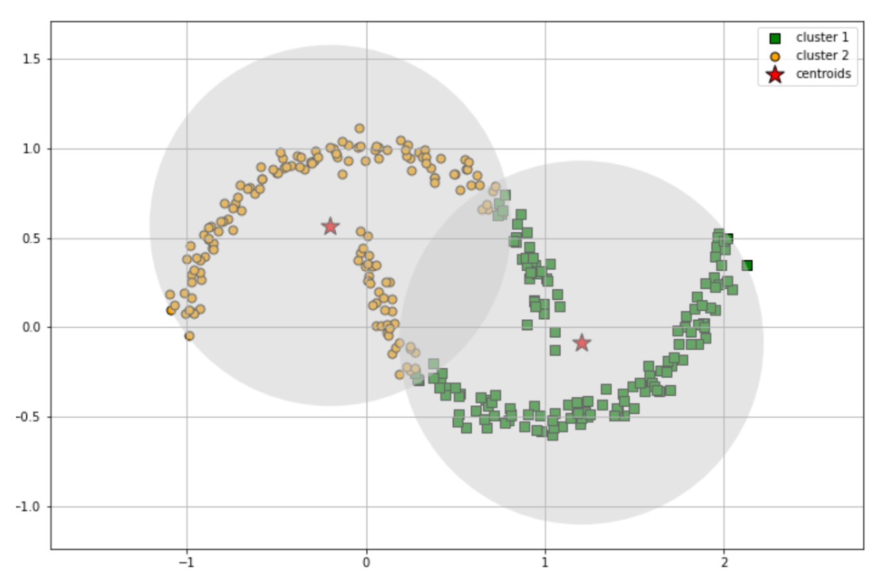
However, when we use DBSCAN, you will see in the following section that it can capture arbitrary shapes of clusters. Below is the step-by-step explanation how the DBSCAN algorithm works:

• First, we need to define a couple of parameters in advance: a threshold distance, let’s call it epsilon, and the number of minimum neighbors in a data point, let’s call it min_samples.
• Now, for each data point, the algorithm will count the neighboring data points that are located within epsilon.
• If the count of neighbors of a data point is higher than min_samples, then this particular data point will be called a core sample. In the DBSCAN algorithm, a core sample means that a data point is located in a highly dense region.
• All of the neighboring points of a core sample will be grouped into one cluster. Meanwhile, if there is any data point that is not considered as a core sample nor being a neighbor of any core sample, then the DBSCAN clustering algorithm will consider this data point as an outlier.

Implementation of DBSCAN Algorithm

Now that we know how the DBSCAN machine learning clustering algorithm works, let’s implement it with Python. To do this, we can use the Scikit-learn library, especially with DBSCAN class. First, let’s generate a dataset for our example.

import numpy as np
from sklearn.cluster import DBSCAN
from sklearn.datasets import make_moons
from sklearn.preprocessing import StandardScaler

X_moon, labels_true = make_moons(
    n_samples=300,  noise = 0.05, random_state=0
)

And below is the visualization of the resulting data points from the code snippet above:

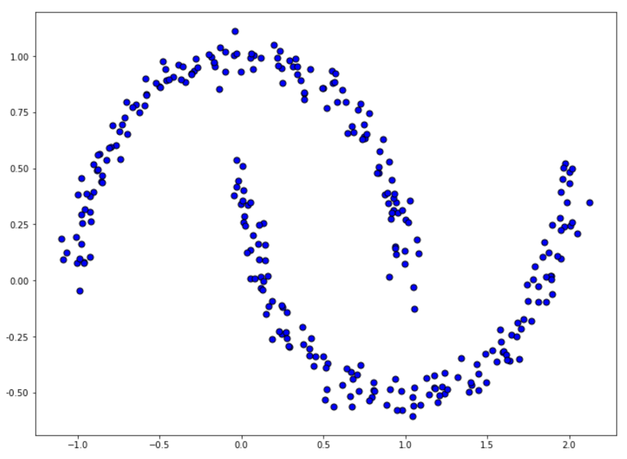
To implement DBSCAN, first, we need to standardize our data, and then call DBSCAN class from the Scikit-learn library. For our example, we’re going to define the eps value, which is the threshold distance, to 0.3 and the number of minimum neighbors (min_samples) to be 10.

X_moon = StandardScaler().fit_transform(X_moon)
db = DBSCAN(eps=0.3, min_samples=10).fit(X_moon)

After we train our DBSCAN model on the training data, then we can check to which cluster each of our data points belongs. To do this, we can use labels_ method as you can see in the following code snippet:

db.labels_

Output: array([0, 1, 1, ..., 0, 1, 0, 0, 0])

The result that we will get is an array with the shape equal to the number of data points. Each element of the array is the label of the cluster to which your data point belongs. In our example use case above, the DBSCAN algorithm converges into the result that the optimum number of clusters would be 2, hence the value of either 0 or 1 in each element of the array.

However, if we have outliers in our dataset, then the DBSCAN algorithm will give them -1 as the label.

Finally, the visualization of the clustering process using DBSCAN can be seen below:

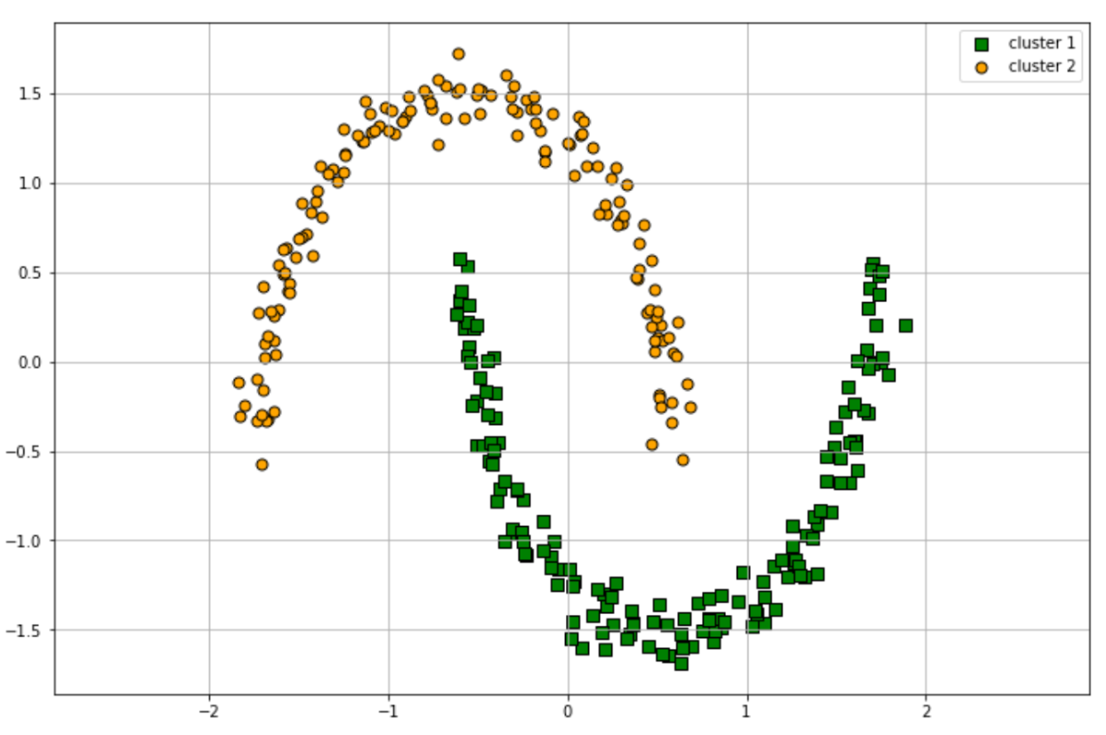
As you might have noticed from the working process of the DBSCAN clustering algorithm, there are two important parameters that we can fine-tune in order to improve the performance of the model, which are the epsilon value and the minimum neighbors value. In a more complex dataset, fine-tuning of these two parameters will be important to improve the quality of the clustering result.

HDBSCAN

There is one additional machine learning clustering algorithm that is basically an extension of the DBSCAN algorithm called HDBSCAN or Hierarchical DBSCAN. This algorithm has a similar workflow in comparison with DBSCAN with one difference: with HDBSCAN, we don’t need to specify the value of parameter epsilon in advance. This is because HDBSCAN will try to find the optimal clusters based on varying distances.

With this feature, HDBSCAN maintains all of the positive things about DBSCAN whilst also being able to identify clusters with varying densities. Thus, the only parameter that we need to define in advance is the minimum cluster size.

HDBSCAN has its own library in Python that we can install via pip. The good thing is, the API of this library is similar to the DBSCAN algorithm that we have implemented above with Scikit-learn. Below is an example of how we can implement HDBSCAN:

import hdbscan
import numpy as np
from sklearn.preprocessing import StandardScaler

hdb = hdbscan.HDBSCAN(min_cluster_size=5, gen_min_span_tree=True).fit(X_moon)

As you can see above, we didn’t explicitly specify the epsilon parameter, as HDBSCAN algorithm doesn’t need a fixed threshold distance value to come up with the optimal clusters. However, we still need to define the minimum cluster size. This parameter defines that if the split occurs when we have fewer points than our minimum cluster size, then instead of splitting them into two different clusters, those data points will be considered to fall out of the cluster.

We can also see to which cluster each data point belongs with label_ method.

hdb.labels_

Output: array([1, 0, 0, ..., 0, 1, 1, 1]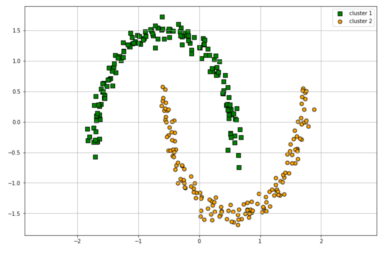

Conclusion

In this article, we have learned about machine learning clustering methods, which is an unsupervised learning method in the machine learning paradigm. Specifically, we now know different algorithms of clustering methods such as k-Means Clustering, Gaussian Mixture Model, Agglomerative Clustering, and DBSCAN.

The k-Means clustering method usually performs well when our data points have a circular shape cluster, plus the workflow of this algorithm is easy to follow. Meanwhile, DBSCAN and Gaussian Mixture Model offer us more flexibility in terms of cluster shape. Agglomerative clustering and DBSCAN are good algorithms to use when we don’t really want to deal with the hassle of finding out the optimal cluster for our use case.