Introduction to Polars: Everything You Must Know?

Big data holds a huge commitment! If you work with a large dataset, you know how even a minor modification in a function can save you hours. Both speed and efficiency are the key factors driving the flow above.

We'll find it out in this article, not just a theory. In this post, we'll take an interview question recently asked by Visa and break down the solutions into codable steps, and in the process, we'll show you how polars works quickly.

It will be informative and give you an edge to use the knowledge for future interviews. So, let’s get started!

Polars & Pandas, and how do you set Polars?

We know that Pandas has a pretty big community and is quite known, but when you generate big datasets, the arrow starts to lag, and in that case, how can we take advantage of Polars? The answer is Polars, which has a super quick Pandas-like library.

Why is it fast? Part of the reason for this is that it will be vectorized, but we will discover all the reasons in the next step.

Normally, you can do it by installing polars like this:

pip install polars

But you don't have to do this manually; if you visit our platform here, you can use polars.

So now you are ready. Let’s see the advantages Polar holds over the Pandas

Why Use Polars Over Pandas?

You already know the biggest reason why Polars used pandas by now. But there are more reasons just like that. Let’s see them.

1. Which one is faster?

While pandas is single-threaded, polars executes all parallel operations on all your CPU cores. That makes it faster for a larger set of data.

2. Low Memory Usage means low cost.

Polars uses a columnar memory layout instead of single-row execution (pandas). That causes low memory consumption.

3. Lazy Evaluation works like magic!

Execution-wise, Polars is sort of lazy in comparison to Pandas. Polars will not run commands unless commanded to do so. It optimizes and runs queries in one shot, saving time and resources.

4. Built with Rust, Not Python.

Python scores high in usability, while Rust does not. Polars is a highly efficient data processing library that marries Python's usability with Rust's raw power.

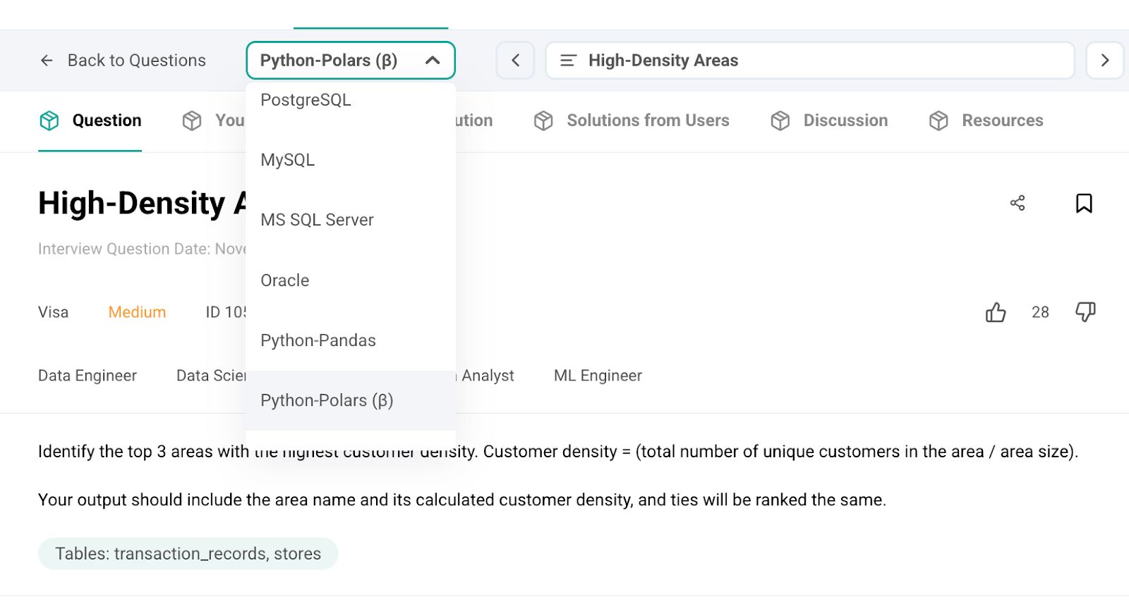
Practice Question: High-Density Areas

Link to this question:https://platform.stratascratch.com/coding/10544-high-density-areas

As you can see from the description above, visa asks us to find the top three areas with the highest customer density. So, we should identify where unique customers cluster the most per unit area. Let’s break down the problem.

Breaking Down the Problem

We have two datasets, transaction_records and stores. Let’s preview them first. Here is the transaction_records.

Here is the stores dataset:

To answer this question, this is what we should do:

1. Combine datasets
2. Count the unique customers
3. Compute the customer's density
4. Rank the areas

Expected Output

Here is the expected output of our question.

Step-by-Step Solution with Polars

Now that we understand the problem let’s solve it step by step using Polars. Each step tackles a specific part of our objective, making the process transparent and efficient.

Step 1: Merging Transaction Records with Store Data

To calculate the customer density, we need to join the dataset first. Since both datasets contain store_id, we can join them using this column. Here is the relevant column.

import polars as pl

merged_data = transaction_records.join(
    stores.select(["store_id", "area_name", "area_size"]),
    on="store_id",
    how="inner"
)

Let’s see how this code works:

• join( ) combines the datasets, ensuring that area_name and area_size are linked to every transaction.
• The how = “inner” ensures only matching store records appear in the final dataset.

Each transaction includes the store’s area details. It allows us to move to the next step.

Step 2: Counting Unique Customers per Area

At this step, we must determine how many unique customers have visited each before calculating the customer density. Here is the relevant code:

unique_customers_per_area = (
    merged_data
    .group_by("area_name")
    .agg(pl.col("customer_id").n_unique().alias("unique_customers"))
)

Let’s see how the code above works:

• group_by("area_name") groups transactions by area.
• .agg(pl.col("customer_id").n_unique()) counts unique customers per area.
• .alias("unique_customers") renames the column for clarity.

At this step, we have a table that tells us how many unique customers exist in each area.

Step 3: Calculating Customer Density

Now, we must calculate the customer density. Density is calculated using

• (total number of unique customers in the area / area size).

This tells us how many unique customers exist per unit area. Here is the relevant code block:

customer_density_data = unique_customers_per_area.join(
    stores.select(["area_name", "area_size"]),
    on="area_name",
    how="inner"
)

customer_density_data = customer_density_data.with_columns(
    (pl.col("unique_customers") / pl.col("area_size")).alias("customer_density")
)

Let’s see what we did with the code block above:

• We merge the unique customer counts with area_size.
• We divide unique_customers by area_size to compute customer_density.

Now, each area has a customer density score. It helps us identify high-density zones.

Step 4: Ranking Areas Using Dense Ranking

Now, we will find the top three areas. So, we rank them based on the customer density, which we just calculated using dense ranking. But you should be careful that tied areas receive the same rank. Here is the relevant code:

customer_density_data = customer_density_data.with_columns(
    pl.col("customer_density").rank("dense", descending=True).alias("rank")
)

Now let’s see what we did here:

• rank("dense", descending=True) assigns the highest density rank 1.
• Tied areas get the same rank instead of skipping numbers.

Each area has a rank, allowing us to filter the top ones. We have one step left.

Step 5: Filtering & Outputting the Top 3 Areas

Now, let’s filter the top 3 areas, select the relevant names, and see the result. Here is the relevant code block:

top_3_areas = customer_density_data.filter(pl.col("rank") <= 3)
final_result = top_3_areas.select(["area_name", "customer_density"])
final_result

Let’s see what we did with the code block above:

• .filter(pl.col("rank") <= 3) keeps only the top 3 ranked areas.
• .select(["area_name", "customer_density"]) keeps only relevant columns.

The final result contains the top 3 areas with the highest customer density!

Running the Complete Polars Code

Now you know how it works, so let’s run the entire code in one go to see how it works from start to finish. Here is the relevant code:

import polars as pl

merged_data = transaction_records.join(
    stores.select(["store_id", "area_name", "area_size"]),
    on="store_id",
    how="inner"
)

unique_customers_per_area = (
    merged_data
    .group_by("area_name")
    .agg(pl.col("customer_id").n_unique().alias("unique_customers"))
)

customer_density_data = unique_customers_per_area.join(
    stores.select(["area_name", "area_size"]),
    on="area_name",
    how="inner"
)

customer_density_data = customer_density_data.with_columns(
    (pl.col("unique_customers") / pl.col("area_size")).alias("customer_density")
)

customer_density_data = customer_density_data.with_columns(
    pl.col("customer_density").rank("dense", descending=True).alias("rank")
)

top_3_areas = customer_density_data.filter(pl.col("rank") <= 3)


final_result = top_3_areas.select(["area_name", "customer_density"])

final_result

Here is the output.

Excellent. As you can see, it matches the expected output.

How Do We Know It's Correct?

• Customer Density is calculated correctly (unique customers ÷ area size)
• Both Area D & Area E have the same rank due to dense ranking in case of ties.
• Correctly filters places ranked top three.

Final Thoughts

Data processing at scale demands both speed and efficiency. Of course, you can process data with other libraries like Pandas or without using a library with custom functions, but would that be logical? Or would it be the best industry practice?

In this article, we introduce polars by using step-by-step real-life interview questions. When learning new concepts, these real-life interview questions will also give you a real-life experience that can be used in your interview process.