Feature Selection Techniques in Machine Learning

We’ll talk about supervised and unsupervised feature selection techniques. Learn how to use them to avoid the biggest scare in ML: overfitting and underfitting.

If you're working with a dataset and trying to build a machine learning model, you probably don't need all the data and columns that feed into your model. Using unnecessary data can confuse the model and lead to undesirable results like overfitting or underfitting.

So, how do you choose the right columns and data that will have the most impact on your model? We’ll answer exactly that question in this article.

Choosing the right feature selection method is like choosing the right weapon in a video game. It completely depends on your data and the goal of the project itself.

The two main categories of feature selection are supervised and unsupervised machine learning techniques. Here’s the overview.

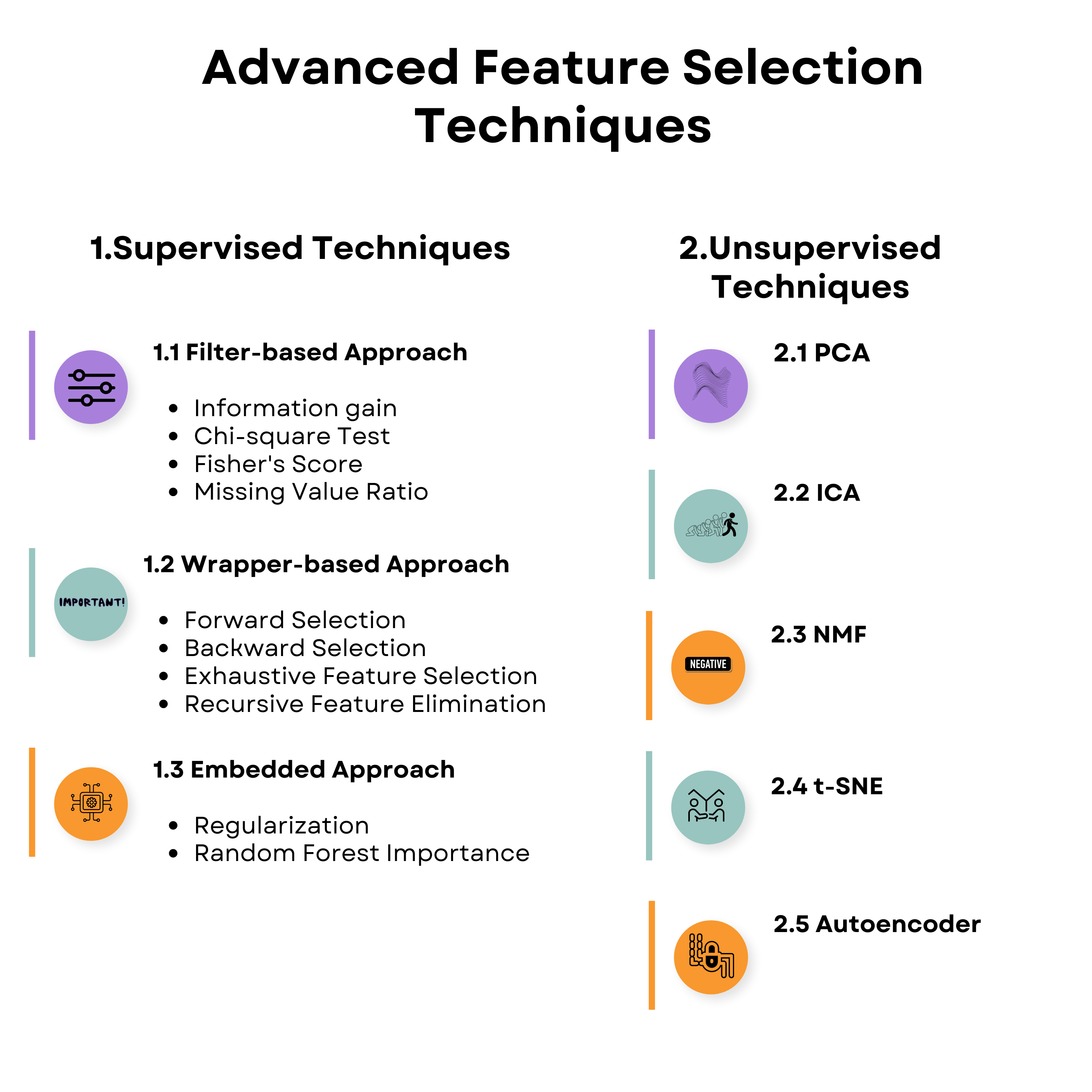
Let’s kick off with supervised learning.

Supervised vs. Unsupervised Learning

Supervised learning means that you're going to use labeled data to train algorithms and predict outputs for new, unseen data. On the other hand, unsupervised machine learning deals with unlabeled data and aims to discover hidden patterns within that data. If you want to go deeper into this, check out our post "Supervised vs Unsupervised Learning".

Supervised Feature Selection Techniques in Machine Learning

Supervised feature selection is a process in machine learning where the selection of relevant features (variables, predictors) in your data is guided by the target variable, i.e., the output you want to predict.

The three supervised feature selection techniques we’ll discuss are filter-based, wrapper-based, and embedded approaches.

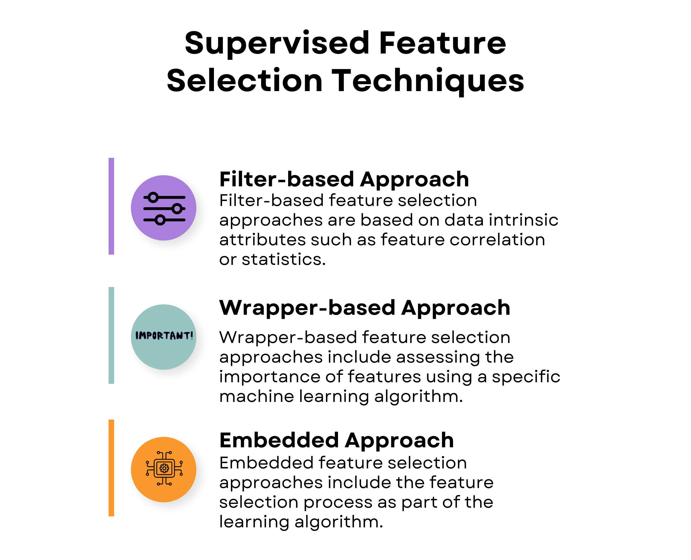
Let’s start with the filter-based approach!

Filter-Based Feature Selection Techniques in Machine Learning

Filter-based approaches assess the value of each feature without considering the performance of a specific machine learning algorithm. You're evaluating just the data itself to understand how the data correlates with each other. Within filter-based approaches, there are four feature selection techniques.

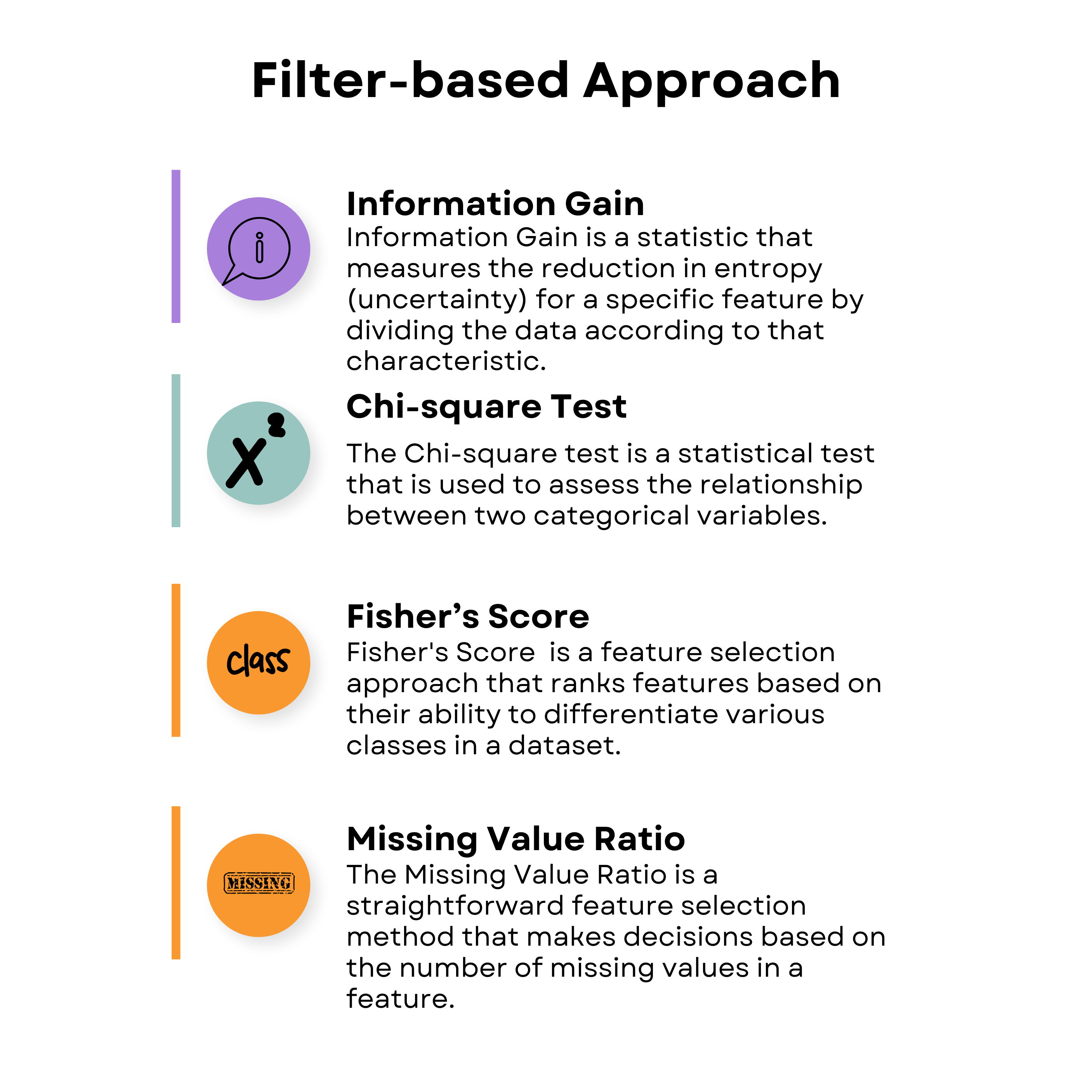
We have also covered filter-based feature selection techniques in this video:

Information Gain

Information Gain is where we look at different things and see which ones are the most helpful for finding answers.

It's like sorting out toys into groups based on their colors or shapes to find the most interesting ones.

Your code might look something like this.

import numpy as np
import matplotlib.pyplot as plt
from sklearn.datasets import load_diabetes
from sklearn.feature_selection import mutual_info_regression

# Load the diabetes dataset
data = load_diabetes()

# Split the dataset into features and target
X = data.data
y = data.target

# Apply Information Gain
ig = mutual_info_regression(X, y)

# Create a dictionary of feature importance scores
feature_scores = {}
for i in range(len(data.feature_names)):
    feature_scores[data.feature_names[i]] = ig[i]
# Sort the features by importance score in descending order
sorted_features = sorted(feature_scores.items(), key=lambda x: x[1], reverse=True)

# Print the feature importance scores and the sorted features
for feature, score in sorted_features:
    print("Feature:", feature, "Score:", score)
# Plot a horizontal bar chart of the feature importance scores
fig, ax = plt.subplots()
y_pos = np.arange(len(sorted_features))
ax.barh(y_pos, [score for feature, score in sorted_features], align="center")
ax.set_yticks(y_pos)
ax.set_yticklabels([feature for feature, score in sorted_features])
ax.invert_yaxis()  # Labels read top-to-bottom
ax.set_xlabel("Importance Score")
ax.set_title("Feature Importance Scores (Information Gain)")

# Add importance scores as labels on the horizontal bar chart
for i, v in enumerate([score for feature, score in sorted_features]):
    ax.text(v + 0.01, i, str(round(v, 3)), color="black", fontweight="bold")
plt.show()

You have your labeled and unlabeled data and run it through the information gain model to evaluate the most important features.

The output then might look something like this.

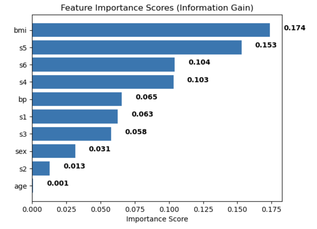
The higher the number you see on the visual, the more important the feature is to understand what leads to a certain outcome—in this case, getting diabetes.

Chi-Squared Test

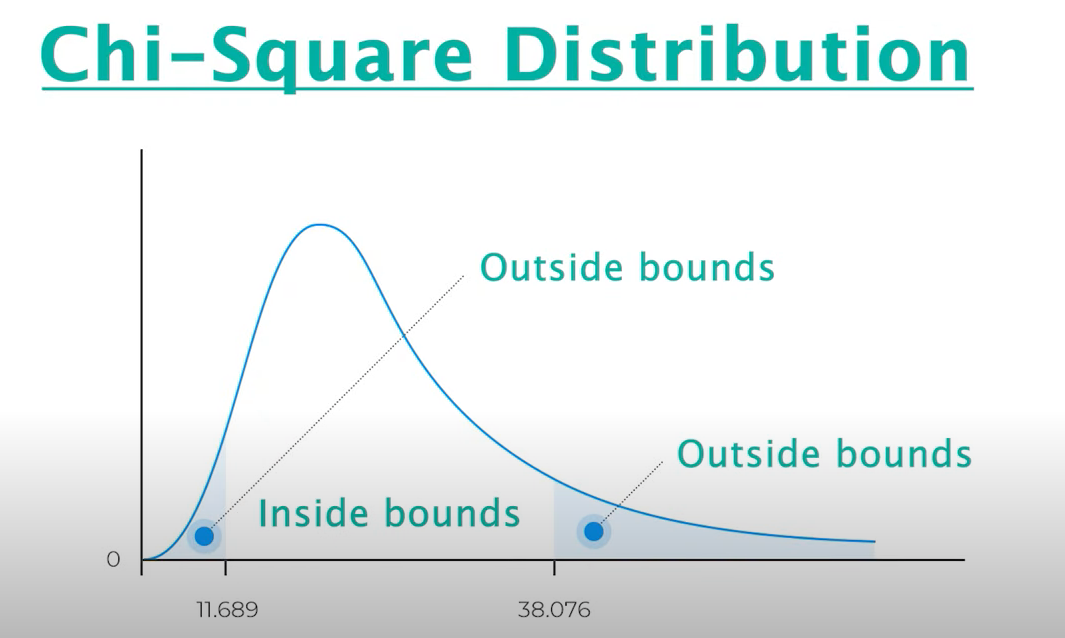
The Chi-Squared Test is a simple statistical test that helps us understand if things are related or just happen by chance.

The formula is:

It's like playing a game to see if two things, like eating corn and feeling happy, correlate.

If the features fall outside the bounds, they are not correlated with each other. If they're inside the bounds, they are correlated.

Fisher's Score

Fisher's Score is a way to find out which things are most important in the group.

It's like giving points to toys based on how special they are. The toys (or, in this case, features) with more points are the ones we should pay attention to because they're the most interesting.

Your code and visualization might look like this.

from skfeature.function.similarity_based import fisher_score
import matplotlib.pyplot as plt
%matplotlib inline

# Calculating scores
ranks = fisher_score.fisher_score(X, Y)

# Plotting the ranks
feat_importances = pd.Series(ranks, dataframe.columns[0:len(dataframe.columns)-1])
feat_importances.plot(kind='barh', color = 'teal')
plt.show()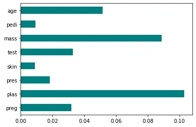

The more points you see on the graph, the more important the feature is.

Missing Value Ratio

The Missing Value Ratio is a way to find out how many things are missing in the group. It's sort of like counting how many puzzle pieces are missing from a puzzle. If there are too many missing pieces, then it might be hard to complete the puzzle and understand the whole picture.

Likewise, if there are too many features that have missing data, the feature itself may not really work for the model.

Let’s now go to the wrapper-based approach!

Wrapper-Based Feature Selection Techniques in Machine Learning

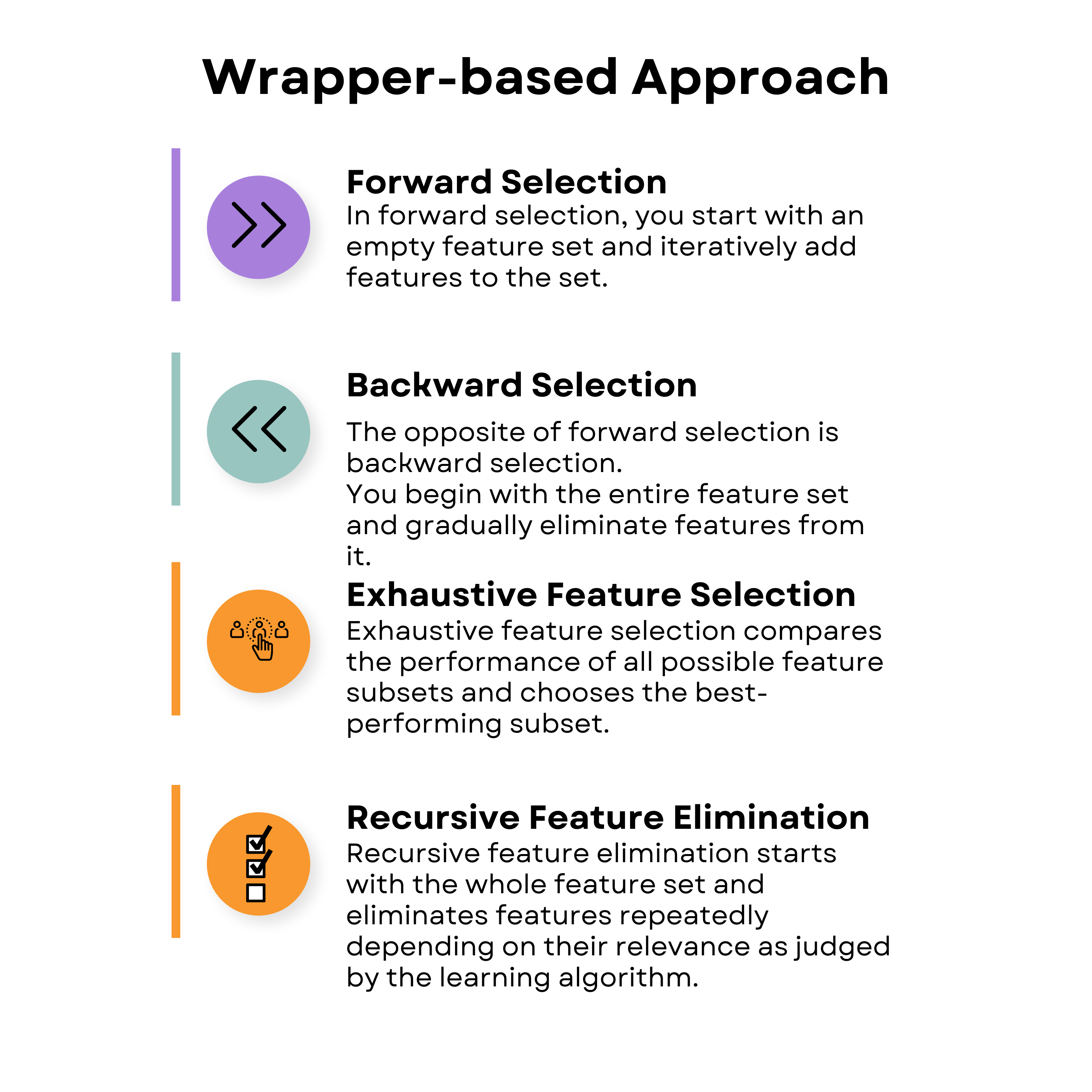
Wrapper-based approaches can be likened to having a friend who tries different toys and tells you which are the most fun to play with. In this case, the 'helper' is a specific machine learning model that you're going to use to determine the most important 'toys' or features in the dataset.

There are four main types of wrapper-based feature selection techniques shown below.

Here's the video where we've covered wrapper-based approaches and embedded approaches in the realm of supervised techniques for feature selection in machine learning.

Forward Selection

Following the toy analogy, you start with one toy and see how much fun it is. Then add another toy and see if it makes things even more fun. Keep adding toys until you have the most fun collection to play with. An example is given using logistic regression to find the best features. A graph shows that with four features, you can achieve an accuracy of 95%.

Here is some code that tries to find the best features using logistic regression.

import numpy as np
import pandas as pd
from sklearn.datasets import load_breast_cancer
from sklearn.linear_model import LogisticRegression
from sklearn.model_selection import train_test_split
from mlxtend.feature_selection import SequentialFeatureSelector as SFS

# Load the breast cancer dataset
data = load_breast_cancer()

# Split the dataset into features and target
X = data.data
y = data.target

# Split the dataset into training and testing sets
X_train, X_test, y_train, y_test = train_test_split(X, y, test_size=0.3, random_state=0)

# Define the logistic regression model
model = LogisticRegression()

# Define the forward selection object
sfs = SFS(model, k_features=5, forward=True, floating=False, scoring="accuracy", cv=5)

# Perform forward selection on the training set
sfs.fit(X_train, y_train)

# Print the selected features
print("Selected Features:", sfs.k_feature_names_)

# Evaluate the performance of the selected features on the testing set
accuracy = sfs.k_score_
print("Accuracy:", accuracy)

# Plot the performance of the model with different feature subsets
sfs_df = pd.DataFrame.from_dict(sfs.get_metric_dict()).T
sfs_df["avg_score"] = sfs_df["avg_score"].astype(float)
fig, ax = plt.subplots()
sfs_df.plot(kind="line", y="avg_score", ax=ax)
ax.set_xlabel("Number of Features")
ax.set_ylabel("Accuracy")
ax.set_title("Forward Selection Performance")
plt.show()

And when we graph the number of features needed to get a specific accuracy in our model, we get this.

The graphic shows that, for example, if you have 4 features, you have an accuracy of around 95%.

Backward Selection

It’s the opposite of forward selection. It begins with the full set of features and then removes features one by one, removing the one that doesn't contribute to the model's accuracy until it gets to an optimal subset of remaining features.

Its visualization looks like this.

It shows that the model accuracy stays stable between 6 and 14 features.

Exhaustive Feature Selection

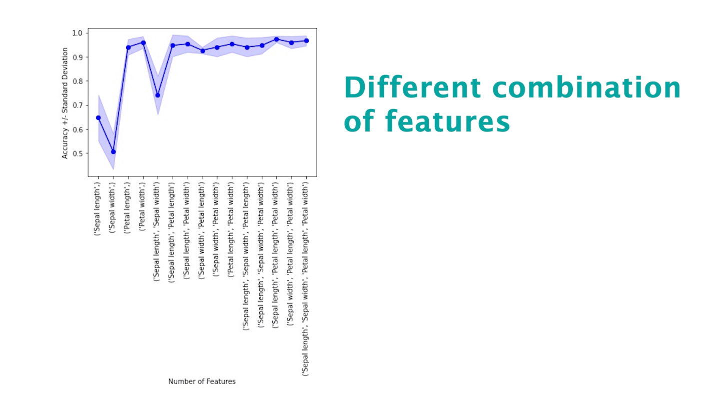
This method evaluates all possible feature combinations to identify the subset that performs best for a specific machine learning model.

Here’s the code that illustrates the implementation.  It uses the ExhaustiveFeatureSelector function using a random forest to do the work.

from mlxtend.feature_selection import ExhaustiveFeatureSelector
from sklearn.ensemble import RandomForestRegressor, RandomForestClassifier
from sklearn.metrics import roc_auc_score

feature_selector = ExhaustiveFeatureSelector(RandomForestClassifier(n_jobs=-1),
           min_features=2,
           max_features=4,
           scoring='roc_auc',
           print_progress=True,
           cv=2)

features = feature_selector.fit(np.array(train_features.fillna(0)), train_labels)

filtered_features= train_features.columns[list(features.k_feature_idx_)]
filtered_features

clf = RandomForestClassifier(n_estimators=100, random_state=41, max_depth=3)
clf.fit(train_features[filtered_features].fillna(0), train_labels)

train_pred = clf.predict_proba(train_features[filtered_features].fillna(0))
print('Accuracy on training set: {}'.format(roc_auc_score(train_labels, train_pred[:,1])))

test_pred = clf.predict_proba(test_features[filtered_features].fillna(0))
print('Accuracy on test set: {}'.format(roc_auc_score(test_labels, test_pred [:,1])))

This technique can be visualized in the following manner. Please note this is just an illustration, not the output of the above code.

Recursive Feature Elimination

This approach starts with a subset of features and then adds or removes features based on their importance.

It can be illustrated like this.

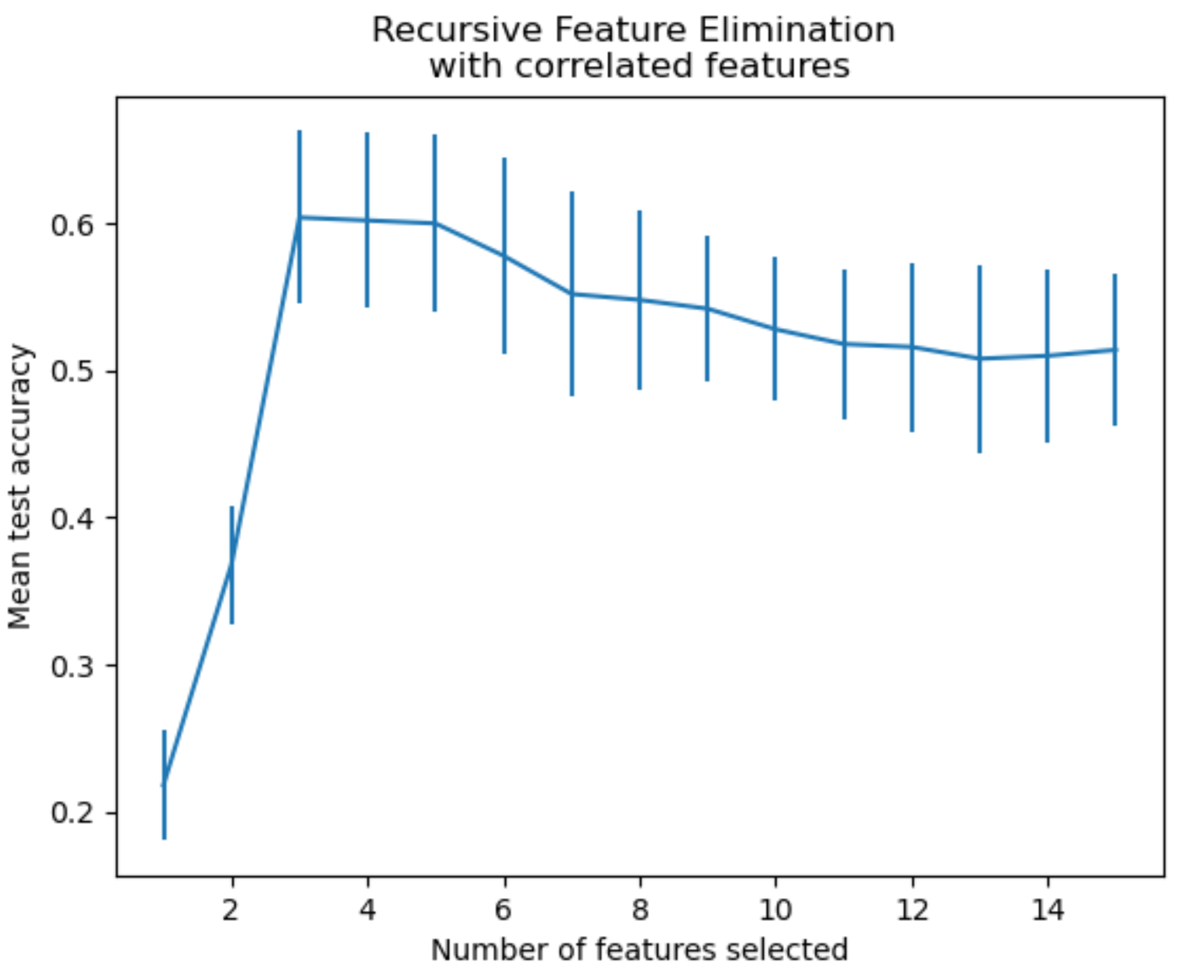
It shows that it adds or removes features based on their importance.

Embedded Feature Selection Techniques in Machine Learning

Embedded approaches is like having a smart robot that can learn and choose the best features for a task all by itself. The robot builds a model as it learns, figures out which features are the most important, and only keeps those.

There are two feature selection techniques in the embedded approach.

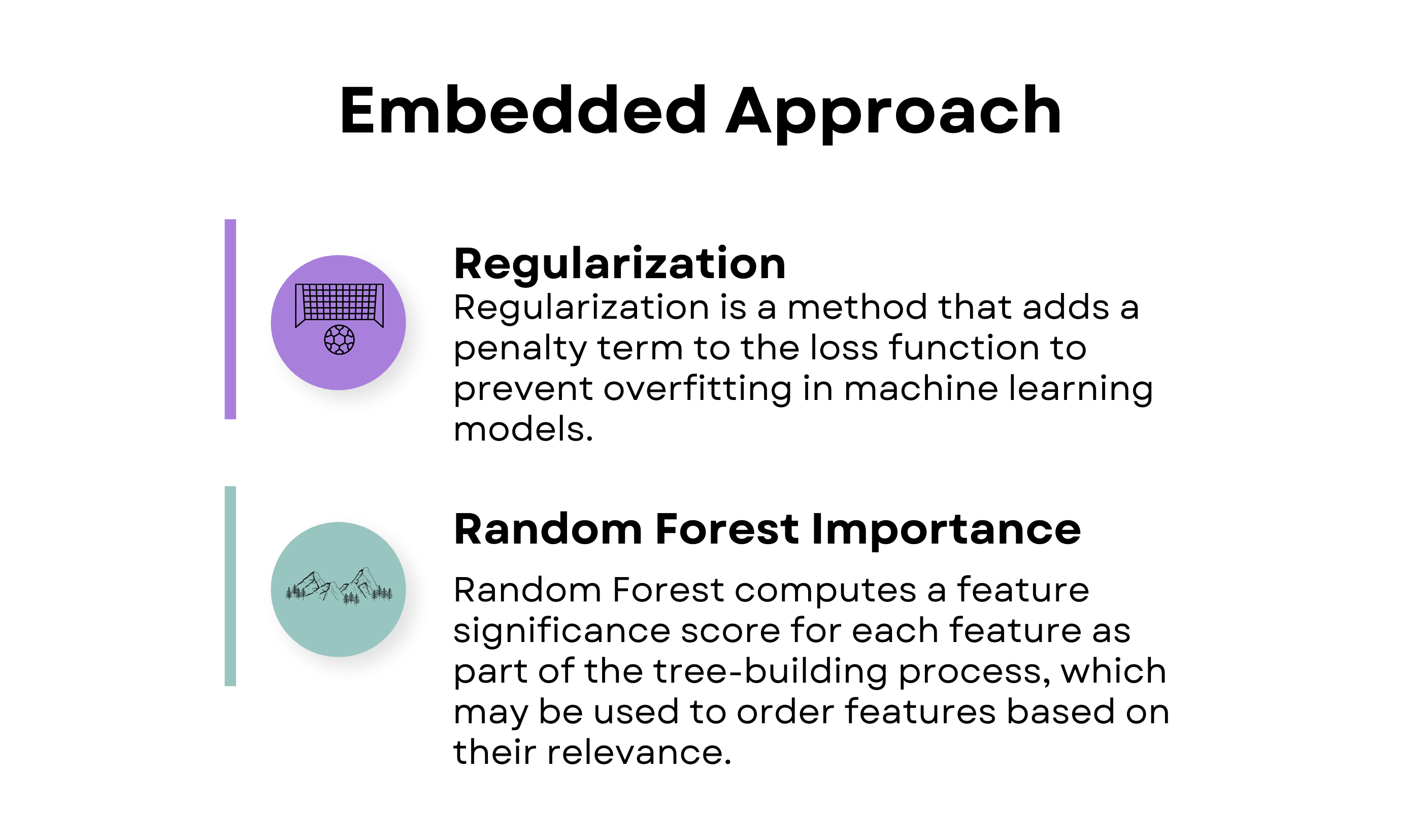
Regularization

This machine learning feature selection technique is like wearing a seat belt while riding a bicycle – it helps you stay safe by preventing you from going too fast and losing control.

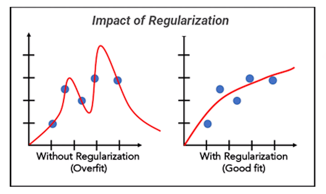
This technique is used to prevent models from becoming too complex and overfitting the data.

Random Forest Importance

Random Forest Importance is like asking a group of friends for advice. Each friend has their own opinion, and some may be more knowledgeable than others.

Random Forest Importance looks at all the opinions from all your different friends (AKA decision trees) and combines them to figure out which factors are the most important in making a decision.

Here’s the code that illustrates this.

import pandas as pd
import numpy as np
from sklearn.ensemble import RandomForestClassifier
from sklearn.model_selection import train_test_split
import matplotlib.pyplot as plt

# Load the Covertype dataset
data = pd.read_csv(
    "https://archive.ics.uci.edu/ml/machine-learning-databases/covtype/covtype.data.gz",
    header=None,
)

# Assign column names
cols = (
    [
        "Elevation",
        "Aspect",
        "Slope",
        "Horizontal_Distance_To_Hydrology",
        "Vertical_Distance_To_Hydrology",
        "Horizontal_Distance_To_Roadways",
        "Hillshade_9am",
        "Hillshade_Noon",
        "Hillshade_3pm",
        "Horizontal_Distance_To_Fire_Points",
    ]
    + ["Wilderness_Area_" + str(i) for i in range(1, 5)]
    + ["Soil_Type_" + str(i) for i in range(1, 41)]
    + ["Cover_Type"]
)

data.columns = cols

# Split the dataset into features and target
X = data.iloc[:, :-1]
y = data.iloc[:, -1]

# Split the dataset into train and test sets
X_train, X_test, y_train, y_test = train_test_split(
    X, y, test_size=0.3, random_state=42
)

# Create a random forest classifier object
rfc = RandomForestClassifier(n_estimators=100, random_state=42)

# Fit the model to the training data
rfc.fit(X_train, y_train)

# Get feature importances from the trained model
importances = rfc.feature_importances_

# Sort the feature importances in descending order
indices = np.argsort(importances)[::-1]


# Select the top 10 features
num_features = 10
top_indices = indices[:num_features]
top_importances = importances[top_indices]


# Print the top 10 feature rankings
print("Top 10 feature rankings:")
for f in range(num_features):  # Use num_features instead of 10
    print(f"{f+1}. {X_train.columns[indices[f]]}: {importances[indices[f]]}")
# Plot the top 10 feature importances in a horizontal bar chart
plt.barh(range(num_features), top_importances, align="center")
plt.yticks(range(num_features), X_train.columns[top_indices])
plt.xlabel("Feature Importance")
plt.ylabel("Feature")
plt.show()

And this is the visualization.

This technique helps us understand which features impact the outcome most.

Unsupervised Feature Selection Techniques

In a nutshell, these are techniques where you’re using an algorithm to find patterns and similarities in data without explicit instructions. In other words, without telling the algorithm what’s good and what’s not, i.e., features are selected without reference to a target variable.

The techniques allow you to explore and discover important data characteristics without using labeled data. These machine learning feature selection techniques are like giving the computer a puzzle and letting it find connections on its own. They’ll organize data and identify similarities without any help from you.

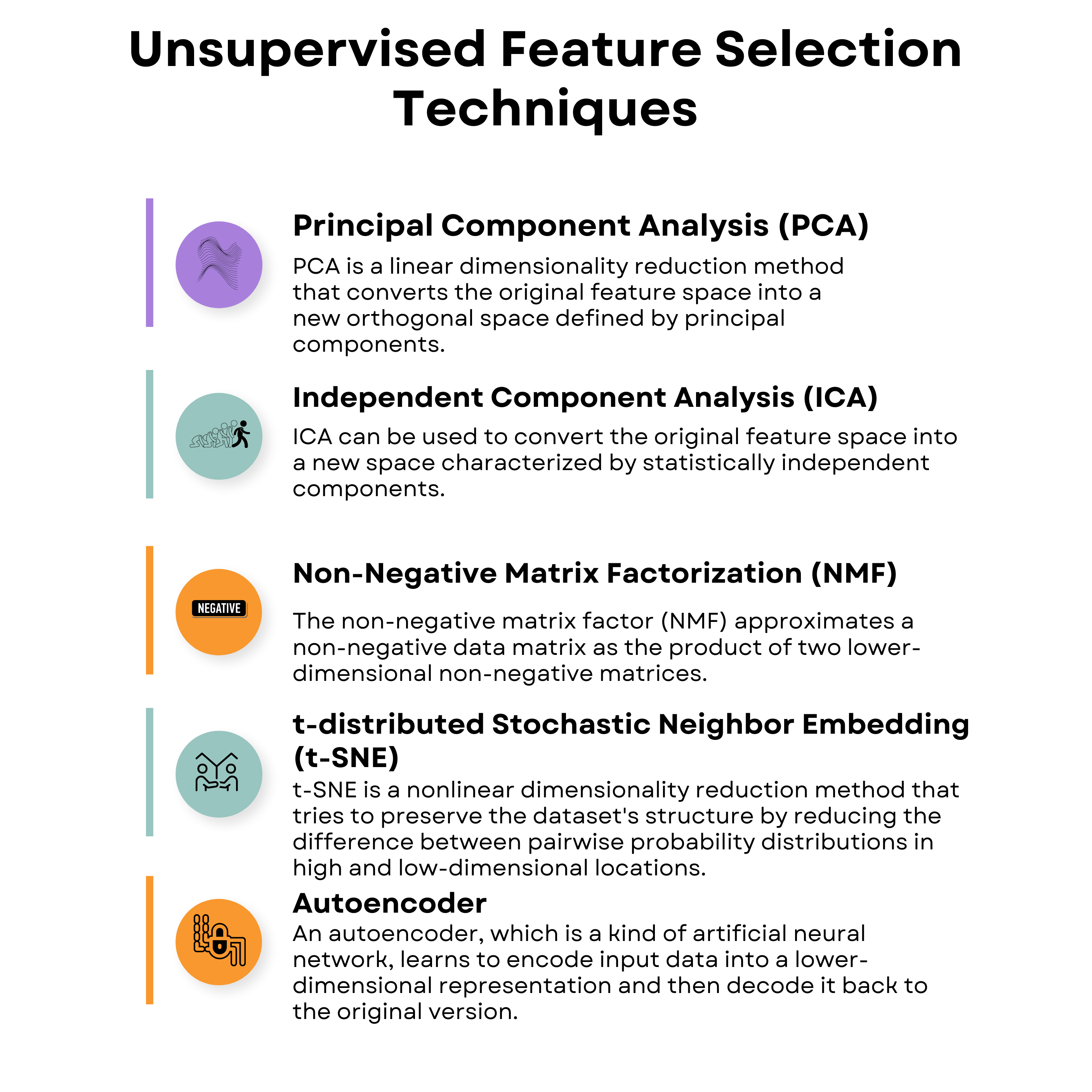
In this part, we’ll cover five unsupervised feature selection techniques in machine learning. The overview is below, familiarize yourself with each approach, and then we explain each one.

Here's the video where we explore the realm of unsupervised feature selection techniques in machine learning.

Principal Component Analysis (PCA)

PCA is a way to understand and simplify data. It helps us find the most important parts of the data. Imagine you have a big picture with lots of details. PCA helps us identify the main shapes or colors that stand out the most. It's like finding the key elements that represent the whole picture without getting lost in the smaller details.

Here’s what your code might look like. Import your data and call the PCA function and you’re done! Programming blindly is easy!

import numpy as np
import pandas as pd
import matplotlib.pyplot as plt
from sklearn.datasets import load_wine
from sklearn.decomposition import PCA
from sklearn.preprocessing import StandardScaler

# Load the Wine dataset
wine = load_wine()
X = wine.data
y = wine.target
feature_names = wine.feature_names

# Standardize the features
scaler = StandardScaler()
X_scaled = scaler.fit_transform(X)

# Perform PCA
pca = PCA()
X_pca = pca.fit_transform(X_scaled)

# Calculate the explained variance ratio
explained_variance_ratio = pca.explained_variance_ratio_

# Create a 2x1 grid of subplots
fig, (ax1, ax2) = plt.subplots(nrows=1, ncols=2, figsize=(16, 8))

# Plot the explained variance ratio in the first subplot
ax1.bar(range(1, len(explained_variance_ratio) + 1), explained_variance_ratio)
ax1.set_xlabel("Principal Component")
ax1.set_ylabel("Explained Variance Ratio")
ax1.set_title("Explained Variance Ratio by Principal Component")

# Calculate the cumulative explained variance
cumulative_explained_variance = np.cumsum(explained_variance_ratio)

# Plot the cumulative explained variance in the second subplot
ax2.plot(
    range(1, len(cumulative_explained_variance) + 1),
    cumulative_explained_variance,
    marker="o",
)
ax2.set_xlabel("Number of Principal Components")
ax2.set_ylabel("Cumulative Explained Variance")
ax2.set_title("Cumulative Explained Variance by Principal Components")

# Display the figure
plt.tight_layout()
plt.show()

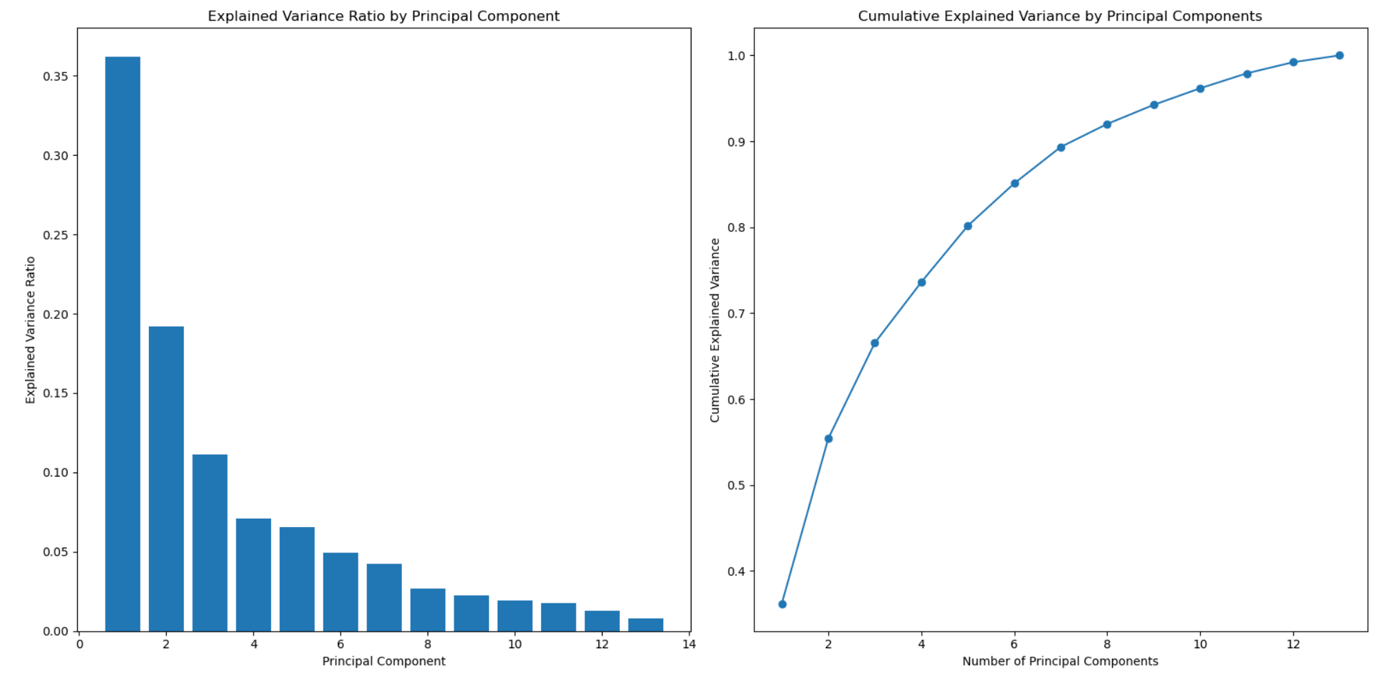
The PCA output is a graph showing the cumulative variance and helps you determine how many features or principal components represent your data. The x-axis represents the number of features, and the y-axis shows the cumulative explained variance.

Independent Component Analysis (ICA)

ICA is a feature selection technique that helps us understand how different things combine together.

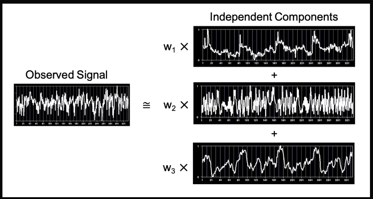
Imagine you have a box of mixed-up sounds like people talking, music playing, cars honking. ICA will help us separate those sounds and figure out what each sound is by itself. It's sort of like listening carefully and picking out the voices or instruments from a noisy crowd to understand what each person or thing is saying or playing.

Here’s the code example. See how easy it is to perform ICA?

>>> from sklearn.datasets import load_digits
>>> from sklearn.decomposition import FastICA
>>> X, _ = load_digits(return_X_y=True)
>>> transformer = FastICA(n_components=7,
...         random_state=0,
...         whiten='unit-variance')
>>> X_transformed = transformer.fit_transform(X)
>>> X_transformed.shape
(1797, 7)

Now, this is what the output might look like.

Non-negative Matrix Factorization (NMF)

NMF is a method that helps us break down big numbers into smaller positive numbers.

Imagine you have a big number representing a whole picture, and you want to understand what parts make up that picture. NMF helps us find smaller positive numbers that, when you combine them, recreate that big number or picture. It's like taking apart a puzzle and then discovering how the smaller pieces fit together to make up that whole picture.

Here’s the code example. Like the other models, this function is also easy to implement.

>>> import numpy as np
>>> X = np.array([[1, 1], [2, 1], [3, 1.2], [4, 1], [5, 0.8], [6, 1]])
>>> from sklearn.decomposition import NMF
>>> model = NMF(n_components=2, init='random', random_state=0)
>>> W = model.fit_transform(X)
>>> H = model.components_

You might end up with the following output.

T-distributed Stochastic Neighbor Embedding (t-SNE)

T-SNE is a machine learning technique that helps us understand how things are related to each other.

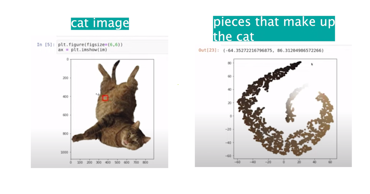
Imagine you have a bunch of pictures of animals, and you want to see which ones are similar to each other. Well, t-SNE helps us create a map where similar animals are placed closer together. T-SNE helps us visualize and explore similarities.

Here’s the code! Again, super easy to call the function and implement the model.

>>> import numpy as np
>>> from sklearn.manifold import TSNE
>>> X = np.array([[0, 0, 0], [0, 1, 1], [1, 0, 1], [1, 1, 1]])
>>> X_embedded = TSNE(n_components=2, learning_rate='auto',
...                   init='random', perplexity=3).fit_transform(X)
>>> X_embedded.shape
(4, 2)

The output would look something like this.

Autoencoder

An autoencoder is a type of artificial neural network that learns how to copy things.

Imagine you have a drawing of an animal, and you want the machine to learn how to draw it by itself. An autoencoder helps the machine learn by giving it the drawing and then asking to create a copy. It's like teaching the machine how to imitate the drawing so it'll learn to draw the animal all by itself.

Autoencoders are useful for teaching machines to understand and recreate things like drawing pictures or images.

Here’s a code that shows you how to implement an autoencoder.

input_size = 784
hidden_size = 128
code_size = 32

input_img = Input(shape=(input_size,))
hidden_1 = Dense(hidden_size, activation='relu')(input_img)
code = Dense(code_size, activation='relu')(hidden_1)
hidden_2 = Dense(hidden_size, activation='relu')(code)
output_img = Dense(input_size, activation='sigmoid')(hidden_2)

autoencoder = Model(input_img, output_img)
autoencoder.compile(optimizer= 'adam', loss='binary_crossentropy')
autoencoder.fit(x_train, x_train, epochsfs)

And here’s the output.

Conclusion

In conclusion, feature selection is a vital process in machine learning that involves identifying the most impactful data for model accuracy.

This article has provided a comprehensive overview of both supervised and unsupervised feature selection techniques, including filter-based, wrapper-based, and embedded approaches.

All these techniques can help avoid overfitting and underfitting, two of the most significant challenges in machine learning.

Now, it’s up to you and your project which feature selection techniques you’ll use.