A Complete Guide to Quick Sort Time Complexity


Categories:
 Written by:
Nathan Rosidi
Quick Sort: A fast algorithm that improves time complexity using pivot-based partitioning and recursion by carefully selecting pivots and structuring the array.
Have you ever considered a way to efficiently sort large datasets without using much additional space? One of the most famous and widely used algorithms, Quick Sort, guarantees precisely that.
In this article, I will take you through Quick Sort, its time complexities, and approaches, which can be called performance optimization.
Explanation of Quick Sort as a Popular Sorting Algorithm
Quick Sort composes the list into two parts, the Left and right sides. This is followed by reordering these messages. Then, they apply this Process to the Sub-array, which gives us a Sorted Array.
Key Components
The efficiency of Quick Sort heavily depends on three key components:
Pivot Selection
The choice of pivot is significant. It can be the first, the last, the middle of all elements, or randomly chosen. Quick Sort can be prolonged if you choose a bad pivot.
Here's an example of using the last element in an array as the pivot.
arr = [10, 7, 8, 9, 1, 5]

def choose_pivot(arr):
    pivot = arr[-1]  # Choosing the last element as the pivot
    return pivot

pivot = choose_pivot(arr)
print("Chosen pivot:", pivot)
Here is the output.


Here, we choose the last element of the array, which is 5, as the pivot.
Partitioning
Once a pivot is selected, the next step will be to place an element less than that of the pivot at one side and greater elements on the other.
Here’s how the partitioning process works on the array.
def partition(arr, low, high):
    pivot = arr[high]
    i = low - 1

    for j in range(low, high):
        if arr[j] <= pivot:
            i += 1
            arr[i], arr[j] = arr[j], arr[i]

    arr[i + 1], arr[high] = arr[high], arr[i + 1]
    return i + 1

pi = partition(arr, 0, len(arr) - 1)
print("Array after partitioning:", arr)
Here is the output.


The array is partitioned around the pivot 5, resulting in [1, 5, 8, 9, 7, 10].
Recursive Sorting
So now we will recursively call quick sort on both the sub-array part before that pivot and the sub-part after it. This step is repeated to sort the whole array.
Quick Sort is a recursive algorithm that calls it on smaller partitions of the entire array. As such, we print the array at each recursive level that loops through different parts of an initial input list. So, we have different outputs as each sub-array is sorted independently.
def quick_sort(arr, low, high):
    if low < high:
        print("Array before recursive step:", arr[low:high+1])  # Show sub-array before sorting

        pi = partition(arr, low, high)
        quick_sort(arr, low, pi - 1)
        quick_sort(arr, pi + 1, high)

        print("Array after recursive step:", arr[low:high+1])
arr = [10, 7, 8, 9, 1, 5]

quick_sort(arr, 0, len(arr) - 1)
print("Sorted array:", arr)
Here is the output.

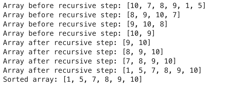
Quick Sort works with sub-arrays, so it will show various orders of partitions as Quick Sort processes different parts of the array:
- Array before recursive step: This will display an array sorted by the current recursion call.
- Array after recursive step: Indicates the part of the array after all recursion has been done in this sub-array
Example of Quick Sort in Action
This section will demonstrate how Quick Sort works on a different unsorted array. This time, we’ll use the array [12, 4, 7, 9, 1, 15, 3].
Here’s how Quick Sort works step by step on this new array:
def partition(arr, low, high):
    pivot = arr[high]
    i = low - 1

    for j in range(low, high):
        if arr[j] <= pivot:
            i += 1
            arr[i], arr[j] = arr[j], arr[i]

    arr[i + 1], arr[high] = arr[high], arr[i + 1]
    return i + 1

def quick_sort(arr, low, high):
    if low < high:
        pi = partition(arr, low, high)

        # Recursively sort elements before and after partition
        quick_sort(arr, low, pi - 1)
        quick_sort(arr, pi + 1, high)
arr = [12, 4, 7, 9, 1, 15, 3]

print("Array before sorting:", arr)
quick_sort(arr, 0, len(arr) - 1)
print("Sorted array:", arr)
Here is the output.


Here is the explanation of the code above;
- Initial Array: The array is unsorted at the beginning: [12, 4, 7, 9, 1, 15, 3].
- First Partition: Let’s select the pivot as the last element, 3, and partition the array around it. The result is [1, 3, 7, 9, 12, 15, 4].
- Recursive Sorting: Quick Sort is applied recursively to both sub-arrays:
- Left Sub-array ([1, 3]): This is already sorted.
- Right Sub-array ([7, 9, 12, 15, 4]): Quick Sort selects a new pivot and recursively sorts the elements.
- Recursive Steps:
- After sorting left and right sub-arrays, you will get the final sorted array [1, 3, 4, 7, 9, 12, 15].
Time Complexity Analysis
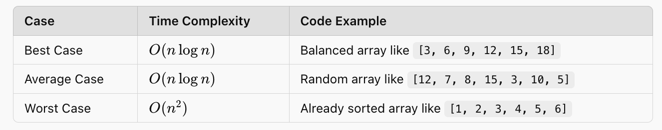
The time complexity of Quick Sort depends on the pivot method and the structure of the array that needs to be sorted. Here are code examples of Best-Case, Average-Case, and Worst-case scenarios with explanations.
Best-Case Time Complexity
It is best when the pivot divides the array into almost two equal parts at each recursive step. This happens if we choose pivots, which always split the array in half.
For example, if our array is perfectly balanced, we have the following:
arr = [3, 6, 9, 12, 15, 18]
quick_sort(arr, 0, len(arr) - 1)
print("Sorted array (Best Case):", arr)
Here is the output.


Explanation:
- In this scenario, the pivot will divide the array into almost equal two parts each time.
- This will minimize the recursion depth, giving us O(nlogn)O(n \log n) time complexity.
Average-Case Time Complexity
Quick Sort works well when the data is not in sorted order, or the pivot that we choose for the sorting purpose is randomly seaborn, which is the most common and cool case for Quick Sort.
A more applaudable realistic average case:
arr = [12, 7, 8, 15, 3, 10, 5]
quick_sort(arr, 0, len(arr) - 1)
print("Sorted array (Average Case):", arr)
Here is the output.

Explanation:
- In the following, we shuffle an array of size 50, and a perfect pivot does not divide evenly.
- However, that is okay, and the average complexity will still be around O(nlogn)O(n \log n)O(nlogn), as long as we limit our recursion!
Worst-Case Time Complexity
The worst case occurs when the pivot selection results in highly unbalanced partitions. For example, almost every time, a sorted or reverse-sorted array is recursively halved by choosing its smallest or largest element as the (worst possible) pivot.
Here is an example of quick sort on a presorted array where the pivot each time we select the last element:
arr = [1, 2, 3, 4, 5, 6]
quick_sort(arr, 0, len(arr) - 1)
print("Sorted array (Worst Case):", arr)
Here is the output.


Explanation:
- The problem is the pivot divide lets every recursion be reduced by one only, with a very deep down to the bottom.
- This gives you the worst time complexity of O(n2)O(n^2)O(n2).
Here is the summary.

Factors Affecting Time Complexity
Many factors can affect the time complexity for Quick Sort, such as which element is selected to choose the pivot and partition algorithm. Knowing these factors can improve the algorithm's performance.
The choice of pivot is responsible for performance optimization in Quick Sort. Different pivot selections can significantly change the algorithm's efficiency.
One common way to solve it is by selecting a random pivot. This will prevent the worst-case scenario, in which the pivot is always the most minor or most significant element. Here is the code.
import random

def random_pivot(arr, low, high):
    pivot_index = random.randint(low, high)
    arr[pivot_index], arr[high] = arr[high], arr[pivot_index]  # Swap the pivot with the last element
    return partition(arr, low, high)

def quick_sort_random(arr, low, high):
    if low < high:
        random_pivot(arr, low, high)
        pi = partition(arr, low, high)
        quick_sort_random(arr, low, pi - 1)
        quick_sort_random(arr, pi + 1, high)

arr = [12, 7, 8, 15, 3, 10, 5]
quick_sort_random(arr, 0, len(arr) - 1)
print("Sorted array with random pivot:", arr)
Here is the output.


Selecting a random pivot mitigates the abuse of weak partitions for a long time, making the algorithm more efficient in best-case scenarios where the input is ordered or has some order.
This helps alleviate the chance of worst-case O(n2)O(n^2)O(n2) performance towards a more likable figure, about what we are used to knowing as O(nlogn).
Partitioning Methods
The next thing that is necessary for the performance of Quick Sort is how you partition the array after selecting your pivot element. The standard partition places the items less than pivot to its left and more significant aspects to its right.
Lomuto partitioning is an easy way to partition and is very widely used. This means the element at the index last will be our pivot. Here is the code.
def lomuto_partition(arr, low, high):
    pivot = arr[high]
    i = low - 1

    for j in range(low, high):
        if arr[j] <= pivot:
            i += 1
            arr[i], arr[j] = arr[j], arr[i]

    arr[i + 1], arr[high] = arr[high], arr[i + 1]
    return i + 1
def quick_sort_lomuto(arr, low, high):
    if low < high:
        pi = lomuto_partition(arr, low, high)
        quick_sort_lomuto(arr, low, pi - 1)
        quick_sort_lomuto(arr, pi + 1, high)
arr = [9, 4, 6, 2, 10, 8]
quick_sort_lomuto(arr, 0, len(arr) - 1)
print("Sorted array with Lomuto partition:", arr)
Here is the output.

Explanation
- While Lomuto partitioning is concise, this approach may need to be more efficient if the pivot always produces imbalanced partitions.
- It is an easy way to go and can be performed in most cases with reasonable accuracy if a decent pivot selection strategy, like random pivoting, etc., is used along with it, as counseled here.
Optimizing Quick Sort
Proper optimization can prevent Quick Sort's worst-case performance and hence improve its overall efficiency. You can get more stable results by choosing the optimal pivot and combining Quick Sort with other sorting algorithms. In this article, we will illustrate two popular optimization methods: select pivot and hybrid.
Choosing the Right Pivot
The pivot is what makes Quick Sort efficient. Picking a bad pivot, for example, by always choosing the smallest or largest element, will degrade the algorithm's performance to O(n2)O(n2)O(n2). We have many techniques for choosing a more accurate pivot pivot for better sorting.
Quick Sort is optimized by a median-of-three pivot strategy. This strategy improves Quick Sort by choosing an excellent random Pivot element and partitioning the array accordingly. This avoids the risk of worst-case performance tail latency.
def median_of_three(arr, low, high):
    mid = (low + high) // 2
    candidates = [(arr[low], low), (arr[mid], mid), (arr[high], high)]
    candidates.sort(key=lambda x: x[0])
    median_value, median_index = candidates[1]
    arr[median_index], arr[high] = arr[high], arr[median_index]  # Move median to the pivot position
    return partition(arr, low, high)

def quick_sort_median(arr, low, high):
    if low < high:
        pi = median_of_three(arr, low, high)
        quick_sort_median(arr, low, pi - 1)
        quick_sort_median(arr, pi + 1, high)

arr = [14, 7, 9, 3, 12, 10, 5]
quick_sort_median(arr, 0, len(arr) - 1)
print("Sorted array with median-of-three pivot:", arr)
Here is the output.


Explanation
- Median-of-three pivoting produces more balanced partitions than selecting a fixed element (like the first or last).
- By reducing the likelihood of highly unbalanced splits, this method generally brings performance closer to O(nlogn)O(n \log n)O(nlogn).
Hybrid Approaches
There are many ways to improve Quick Sort, and one of them is a hybrid approach. One common optimization is to switch from a more expensive sorting algorithm, such as Quick Sort, to Insertion Sort, for example, when the size of the array falls below some threshold.
The hybrid approach made Quick Sort both fast and somewhat recursive (and also improved the performance of small arrays, where recursive overhead wasn't necessary).
For example, if you have a threshold (like 10), Quick Sort will use Insertion Sort in these cases when the sub-array size goes below this number.
def median_of_three(arr, low, high):
    mid = (low + high) // 2
    candidates = [(arr[low], low), (arr[mid], mid), (arr[high], high)]
    candidates.sort(key=lambda x: x[0])  # Sort based on the values
    median_value, median_index = candidates[1]
    arr[median_index], arr[high] = arr[high], arr[median_index]  # Move median to the pivot position
    return partition(arr, low, high)

def quick_sort_median(arr, low, high):
    if low < high:
        pi = median_of_three(arr, low, high)
        quick_sort_median(arr, low, pi - 1)
        quick_sort_median(arr, pi + 1, high)

arr = [14, 7, 9, 3, 12, 10, 5]
quick_sort_median(arr, 0, len(arr) - 1)
print("Sorted array with median-of-three pivot:", arr)
Here is the output.


Explanation
- Insertion Sort is efficient for small arrays, typically with fewer than ten elements. The overhead of Quick Sort’s recursion makes it less practical for such small sub-arrays.
- By combining Quick Sort and Insertion Sort, this hybrid approach leverages the strengths of both algorithms to achieve better performance overall.
Key Takeaways for Optimization
- Median-of-Three Pivot: Helps balance partitions and avoid worst-case scenarios.
- Hybrid Approaches: Switching to Insertion Sort improves performance for small arrays, especially those with fewer than ten elements.
Knowing the fundamentals of structured data will also help you in algorithms like quick sort time complexity.
Comparison with Other Sorting Algorithms
Although Quick Sort is very efficient in various use cases, not all sorting problems can be solved using this algorithm. Merge Sort and Heap Sort are two well-known sorting algorithms compared to QuickSort.
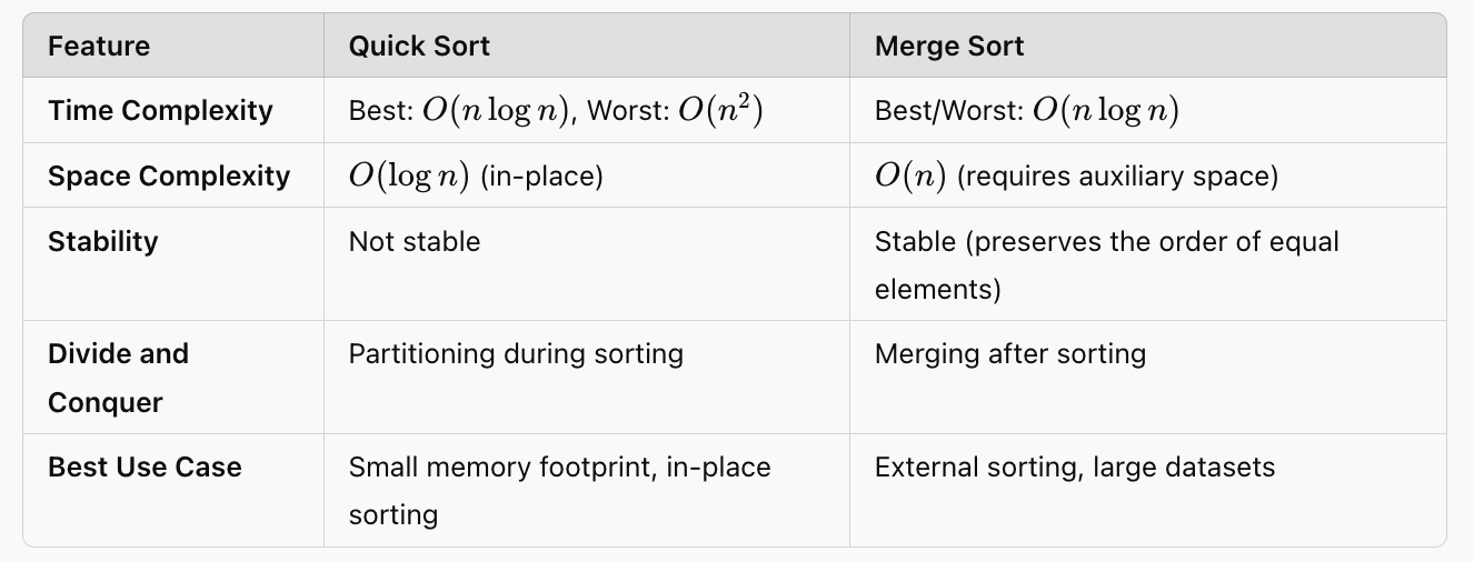
Comparison with Merge Sort
Merge Sort is another divide-and-conquer algorithm like quick sort, but instead of partitioning in a typical fashion, it merges the results back.
Detailed Comparison Between The Two:

Code Comparison:
- In Merge Sort, sub-arrays are formed when the merged array is broken. This mimics the last action for list1 to be intact, making Merge Sorted Arrays such a great way to visualize how we should merge.
- It is more consistent than Quick Sort because Merge Sort always works in O(nlogn) time for all cases but requires additional memory due to the extra merging process.
Practical Example: Merge Sorted Arrays
| Constraints |
|---|
| - `arr1` and `arr2` are both lists of integers. |
| - The input arrays `arr1` and `arr2` are already sorted in ascending order. |
| - The lengths of `arr1` and `arr2` can be different. |
| - The elements in `arr1` and `arr2` can be positive, negative, or zero. |
| - The elements in `arr1` and `arr2` can be repeated. |
| - The maximum length of `arr1` and `arr2` is not specified. |
One of the questions on our platform called Merge Sorted Arrays shows us exactly how the merge is taking place during a theory call to Merge Sort, which can be found here: https://platform.stratascratch.com/algorithms/10385-merge-sorted-arrays
This question asks to merge two sorted arrays, which mimics the main operation of Merge Sort, where two separately sorted pieces of an array are merged back together.
The solution to this problem is as follows-
def merge_sorted_arrays(input):
    arr1 = input[0]
    arr2 = input[1]

    merged_array = []
    i = 0  # Index for arr1
    j = 0  # Index for arr2

    while i < len(arr1) and j < len(arr2):
        if arr1[i] <= arr2[j]:
            merged_array.append(arr1[i])
            i += 1
        else:
            merged_array.append(arr2[j])
            j += 1
    while i < len(arr1):
        merged_array.append(arr1[i])
        i += 1
    while j < len(arr2):
        merged_array.append(arr2[j])
        j += 1

    return merged_array
Here is the test case we will use for this code;

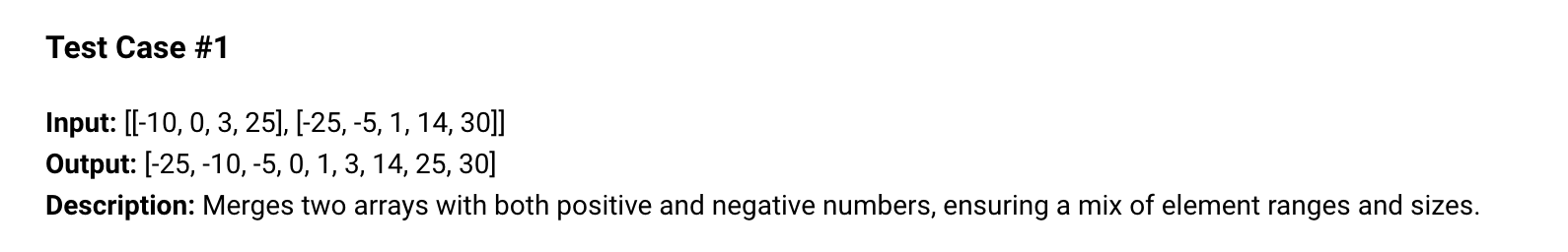
Here is the output.
Expected Output
Official output:
[-25, -10, -5, 0, 1, 3, 14, 25, 30]Official output:
[3, 5, 12, 12, 12, 15, 20, 22, 30]Official output:
[100, 150, 200, 250, 300, 500, 700, 800]As you can see, the expected output matches your output.
Comparison with Heap Sort
Heap Sort is another comparison-based sorting algorithm that builds a heap data structure to sort an array. It’s also an in-place algorithm but with a different approach from Quick Sort.

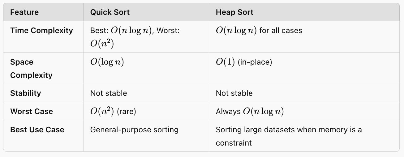
Code Comparison:
- Heap Sort ensures O(nlogn)O(n \log n)O(nlogn) in all cases but is typically slower than Quick Sort due to more data movement during the heapification process.
Here is the code of the Heap sort algorithm.
def merge_sorted_arrays(input):
    arr1 = input[0]
    arr2 = input[1]

    merged_array = []
    i = 0
    j = 0

    while i < len(arr1) and j < len(arr2):
        if arr1[i] <= arr2[j]:
            merged_array.append(arr1[i])
            i += 1
        else:
            merged_array.append(arr2[j])
            j += 1

    while i < len(arr1):
        merged_array.append(arr1[i])
        i += 1

     while j < len(arr2):
        merged_array.append(arr2[j])
        j += 1

    return merged_array
Here is the output.


Summary:
- Heap Sort achieves a predictable O(nlogn)O(n \log n)O(nlogn) running time regardless of the input and is provably more robust in terms of worst-case performance than Quick Sort.
- Quick Sort is generally faster, and fewer comparisons are made. It also performs fewer data movements compared to Heap Sort.
Key Takeaways from the Comparison:
1. Merge Sort guarantees stability and consistent time complexity at the cost of extra memory.
2. Heap Sort is more space-efficient during run-time; it, however, usually performs less efficiently.
3. Quick Sort will require less memory and has an average time complexity of O(n2)O(n^2)O(n2), too, at the expense of having a worst-case scenario with an upper bound on the order if (which can be avoided via various pivot selection strategies).
Practical Considerations
In real-world applications, sorting algorithms like Quick Sort and Merge Sort are selected impeaching based on their nature related to problems and memory, time consumption patterns, and data distribution in order. One use case where sorting is indispensable is reshaping arrays so they are easily digestible for downstream analysis.
Sorted Square Array
| Constraints |
|---|
| - The input array `arr` is a list of integers. |
| - The length of the input array `arr` is not specified, but it should be a non-negative integer. |
| - The elements of the input array `arr` can be positive, negative, or zero. |
| - The input array `arr` may contain duplicate elements. |
| - The input array `arr` may be empty. |
There is one question on our platform called "Sorted Square Array." Here is the link to it.
This problem asks you to return an array of the squares of each element, sorted in non-decreasing order. Let’s see the solution to this question.
def sorted_squares(arr):
    n = len(arr)
    result = [0] * n
    left, right = 0, n - 1
    i = n - 1

    while left <= right:
        if abs(arr[left]) > abs(arr[right]):
            result[i] = arr[left] * arr[left]
            left += 1
        else:
            result[i] = arr[right] * arr[right]
            right -= 1
        i -= 1

    return result
Here is the test case we will use.

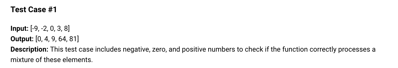
Here is the output.
Expected Output
Official output:
[0, 4, 9, 64, 81]Official output:
[0, 1, 1, 25, 36, 100, 144]Official output:
[0, 1, 2500, 3025, 5625, 9801, 10000]If you want to know more about algorithms, check out this cheatsheet of big-o notation.
Conclusion
Throughout this guide, we explored the Quick Sort algorithm in depth, including its key components, such as pivot selection, partitioning, and recursive sorting.
We also examined how tailored sorting algorithms can benefit real-world problems, such as Sorted Square Array, demonstrating the importance of choosing the right method based on the data's structure.
Share