Decision Tree and Random Forest Algorithm Explained


In this article, we’re going to deeply address everything related to the Decision Tree algorithm and its extension “Random Forest algorithm”.
The Decision Tree algorithm and its extension, i.e., Random Forest are a couple of the most exciting machine learning algorithms out there because these types of algorithms tend to perform superiorly in a machine learning competition in comparison to other algorithms.
Probably you have asked yourself: what is so special about Decision Tree? How does it learn from our data? In this article, we’re going to deeply address everything related to the Decision Tree algorithm and its extension, such as the Random Forest algorithm. Specifically, below are the main talking points that we’re going to cover in this article:
- Decision Tree concept
- Decision Tree learning process
- Decision Tree for multiclass categorical features
- Decision Tree for continuous features
- Decision Tree code implementation
- Drawback of Decision Tree algorithms
- Random Forest concept
- Random Forest data sampling
- Random Forest prediction
- Random Forest code implementation
Without further ado, let’s start with the concept of Decision Tree!
Decision Tree Concept

Based on the name, you might know where the inspiration for this algorithm comes from: yes, a tree. Same as the real tree, a Decision Tree algorithm consists of parts such as root, branch, and leaf. The difference is that in a real tree, you’ll find the root at the bottom of the tree, but in this algorithm, you’ll find the root at the very top of the tree.
Below is the common structure of a Decision Tree algorithm:

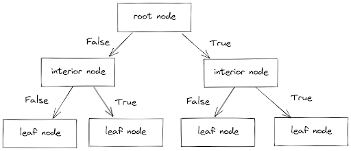
As you can see from the image above, in general, there are three different nodes:
- A root node: normally occupied by the ‘purest’ feature in our dataset (more detailed explanation about this in the next section)
- Several interior nodes: occupied by the rest of the features in our dataset
- Several leaf nodes: consist of the prediction or the outcome of the Decision Tree model.
The different levels of nodes are then connected with a branch. Now, the decision of which branch each data point should go to totally depends on the value of that data point and whether that value fulfills the condition specified in a node. If the value doesn’t fulfill the condition, then it will go to the left branch and vice versa, if it fulfills the condition, then it will go to the right branch.
In each node, each data point must go through this series of True and False conditions until it reaches the leaf node. The leaf node will then give us the prediction of the label of a data point that comes out from the Decision Tree.
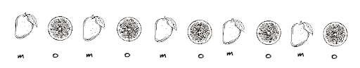
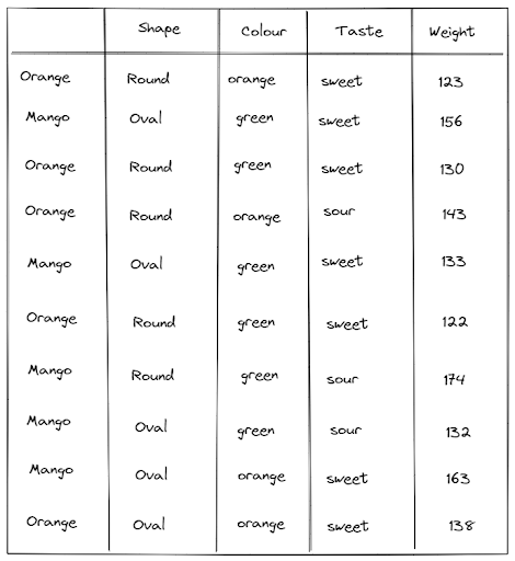
To better understand the concept of a Decision Tree and how it works, let’s take a look at the toy data below:


As you can see above, we have data with ten entries with three different features of fruit, such as shape, color, and taste. Our main purpose with the data above is to classify whether the fruit is mango or orange, given the value of the features.
Each of the features defined in the data above can also be categorized as a categorical feature since each of them has only two possible values, i.e., in the shape feature, the possible value is round or oval, and in the color feature, the possible value is orange and green, and in the taste feature, the possible value is sour or sweet.
With a Decision Tree algorithm, we could end up with a tree structure that looks like either of these:


Not only the two trees as shown above but there are a lot more tree architectures that you might get. Now the question is, how does a Decision Tree algorithm learn from our data such that it will give us the tree architecture that will do the best job to classify our data?
There are two fundamental things about the Decision Tree learning process:
- A Decision Tree algorithm learns by splitting the feature on our data. To decide which feature to split, it will look at the feature with the maximum purity (we will talk about this in detail in the next section)
- There are several criteria that we can adjust to stop the splitting of a Decision Tree during the training process:
- When a node consists of only one class (perfect separation between data points with different classes)
- When further splitting of a Decision Tree will violate the maximum depth of the tree that we set in advance
- When the improvement in the information gain is below the threshold value (we will discuss this as well in the next section)
- When the number of data points in a node is not enough or below the threshold value
Now let’s talk about the learning process of a Decision Tree on our data during the training process.
Decision Tree Learning Process
As mentioned above, a Decision Tree algorithm learns by splitting the feature on our dataset. For each feature on our training set, this algorithm tries to find the purest feature (feature with maximum purity value). The feature with the maximum purity value will then act as a root node. After we have a root node, then the second purest feature will be used as the interior node, and so on.
Now the question is, how does a Decision Tree algorithm measure the purity of each feature? Let’s use the toy dataset that we have introduced in the previous section to make it easier to understand the concept behind it.
In our toy dataset above, we have in total ten entries, which consist of five mangos and five oranges. Let’s say that the goal of our Decision Tree algorithm is to classify whether a fruit is a mango or not. Thus, we can define the fraction of mangos on our dataset to be something like this:

where p_m is the fraction of our data that can be classified as mango.
To measure the purity of a feature, we then can use the so-called entropy function, which has the following form:

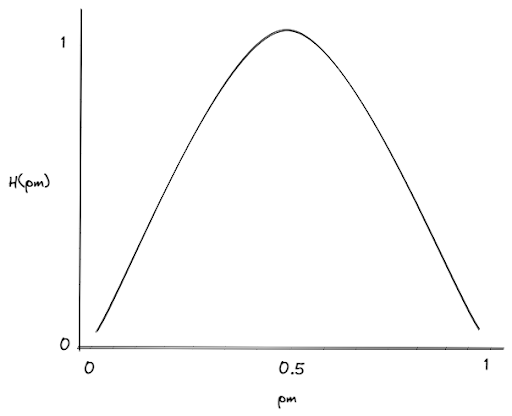
In the image above, H(pm) is the entropy function, which measures the impurity of the feature. The higher the entropy function, the higher the impurity of the feature.
If we have a feature that splits our class into two equal proportions (for example, two mangos and two oranges, then p_m value would be 0.5, which in turn results in H(pm) = 1. This means that this feature is impure, and choosing this feature as a root node would be a poor choice.
On the contrary, if a feature splits our class into heavily unequal proportions (for example, one mango and four oranges), the p_m value would be 0.2, which in turn results in a low value of H(pm). This means that this feature is pure and would be a good choice to be used as a root node.
So now the question is, how can we convert a proportion value (i.e p_m) into its entropy function value (i.e H(pm))?
As we already know, p_m denotes the proportion of our dataset that can be considered a mango. Because of that, we also need to define the proportion of our dataset that is not a mango, and let’s denote this as p_o, which can be defined mathematically as simple as:
If we already know the value of p_m and p_o, then we can compute the corresponding entropy function with the following equation:
To make it easier to understand how a Decision Tree algorithm uses the equation above to choose which feature to split, let’s get back to using our toy dataset that we have introduced earlier.
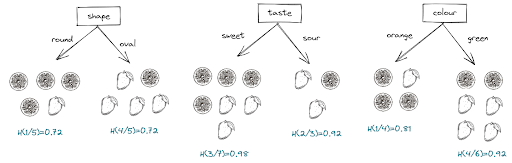
Let’s say that the algorithm now wants to inspect whether the ‘shape’ feature would be a suitable feature to be used to split our data. By looking at our data, below is the visualization of the splitting that the algorithm will get if it uses the ‘shape’ feature as a feature to split our data:

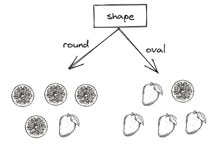
After using the ‘shape’ feature, it turns out that on the left branch (when the shape is round), we get the value of p_m = ⅕ = 0.2, since there is only one mango and the rest are oranges. On the right branch (when the shape is oval), we get the value of p_m = ⅘ = 0.8 since there are four mangos and only one orange.
Putting the p_m value from each branch and plug them into the equation of entropy function, we get:
If we apply the above method to the rest of the features, we will get the following result:

In order to compute the overall entropy of a feature, a weighted method from each of the branches is commonly applied. Below is the general equation on how the weighted method works:
where:
x_left: the fraction of mango on the left branch
x_right: the fraction of mango on the right branch
x_total_left: total data points on the left branch
x_total_right: total data points on the right branch
Implementing the equation above, we get for our ‘shape’ feature the overall entropy function value:
By using the same approach as above, we get for the rest of the features the following overall entropy result:

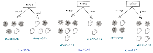
As you can see from visualization above, the feature ‘shape’ has the lowest weighted entropy function, which means that this feature is the purest among other features. However, this weighted entropy function is not the final number that our Decision Tree algorithm uses to choose which feature to split.
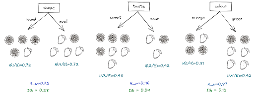
The final value that our Decision Tree algorithm will use is called the information gain. The formula of information gain is:
where H(p_m)_root is the overall entropy of our dataset at the root. In our example, we have ten entries in total, five of which being mangoes. Because of that, we can define the entropy function at root as:
Now that we have the entropy function for our root node, we can compute the information gain for ‘shape’ feature as follows:
With a similar approach, we finally get the information gain for all of the features as can be seen in the following visualization:

The same learning process will be repeated in the next level with the other features (taste and color) until one of the criteria that we have set in advance has been fulfilled, such as:
- When a node consists of only one class (perfect separation between data points with different classes)
- When further splitting of a Decision Tree will violate the maximum depth of the tree that we set in advance
- When the improvement in the information gain is below the threshold value
- When the number of data points in a node is not enough or below the threshold value
Decision Tree Code Implementation
Now that we know about the Decision Tree learning process, let’s implement it in code with the exact same data as we have above. To build and train the Decision Tree model, we will use the scikit-learn library. In the end, we will visualize the decision logic of our model.
First, we can create our data as shown below:
import pandas as pd

shape = ['round', 'oval', 'round', 'round', 'oval', 'round', 'round', 'oval', 'oval', 'oval']
colour = ['orange', 'green', 'green', 'orange', 'green', 'green', 'green', 'green', 'orange', 'orange']
taste= ['sweet', 'sweet', 'sweet', 'sour','sweet', 'sweet', 'sour', 'sour', 'sweet', 'sweet']

label = ['orange','mango','orange', 'orange','mango', 'orange', 'mango', 'mango', 'mango', 'orange']

data = {'shapes': shape, 'colour': colour, 'taste': taste}
df_features = pd.DataFrame(data=data)
Each entry of our data is in a string format (‘sweet’, ‘round’, ‘green’), and we need to transform each of them into a numeric value, as an example, ‘sweet’ would be 0 and ‘sour’ would be 1 so that they can be used as features for our Decision Tree model.
shape = pd.DataFrame(df_features.shapes.replace(['round','oval'],[0,1]))
colour = pd.DataFrame(df_features.colour.replace(['orange','green'],[0,1]))
taste = pd.DataFrame(df_features.taste.replace(['sour','sweet'],[0,1]))
df_features = pd.concat([shape, colour, taste], axis=1)
Next let’s build and train our model with the scikit learn library. We literally only need to few lines of code to do these two things:
from sklearn.tree import DecisionTreeClassifier, plot_tree

decision_tree = DecisionTreeClassifier(random_state=2, criterion='entropy')
decision_tree.fit(df_features, label)
And that’s basically it.
Now that we have trained our model, we can visualize the decision logic of how it splits our feature with the following code:
fig, ax = plt.subplots(figsize=(12, 9))
plot_tree(decision_tree, ax= ax, feature_names=['shape','colour','taste'])
plt.show()

As you can see above, our Decision Tree model used the ‘shape’ feature to split our data in the root node. And this is totally expected as we also found out by computing manually that the ‘shape’ feature will result in the best information gain for our model in the root node compared to other features. From the visualization, this feature has an entropy of 0.722, exactly the same as what we have manually computed in the previous section.
Decision Tree for Multiclass Categorical Feature
In our example about fruit classification above, all of our features can be classified as binary features, i.e., each of them only has two possible values. However, what if our features have more than two possible values? What if in our ‘color’ feature, we don’t only have green and orange as the option, but also red, as an example.
Whenever we use a Decision Tree algorithm, and we have categorical features with more than two possible values, then we need to use an encoding method called one-hot encoding. This method gives a binary representation of each possible value in a feature.
As an example, let’s say that our ‘color’ feature has three possible values: orange, green, and red, as you can see below:


with one-hot encoding, then we have a binary representation of each value in our ‘color’ feature, as shown in the visualization below:

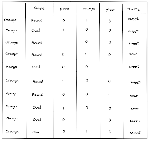
As you can see, now after one-hot encoding, we no longer have a ‘color’ feature, but instead, each of the possible values in our ‘color’ feature becomes a new feature. After we transform our feature with one-hot encoding, then our Decision Tree algorithm will proceed with the learning process described in the previous section.
Decision Tree for Continuous Value
We have covered the situation where the features are categorical features, i.e., where they have a distinctive set of values. The next question would be: what if our feature is continuous, i.e., it can take an infinite number? To illustrate a continuous feature, let’s take a look at below.

As you can see from our modified dataset above, we have a new feature, which is the weight of the fruit measured in grams. The thing about the weight is that it can take any number, and it doesn’t have a discrete value. Thus, this ‘weight’ feature can be classified as a continuous feature.
If we have a continuous feature, the Decision Tree algorithm will look at our feature like this:


In general, the concept of the Decision Tree algorithm if we have a continuous feature is the same as if we have a categorical feature. It will transform our continuous value into a binary representation such that a data point can go either to the left branch or right branch, depending on whether that data point fulfills a particular condition.
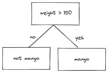
In terms of continuous feature, the Decision Tree algorithm will try to find a value of our feature that will give the best information gain, as you can see in the example below:


Although a Decision Tree algorithm will take a look at the information gain at more splitting points, for the sake of simplicity let’s only consider two splitting points, one at 135 grams and another at 150 grams. To decide which one has the better information gain, we use the same formula as before:
In the end, the splitting point which gives the best information gain will be chosen. Let’s say that the splitting point at 150 gives the best information gain, then the logic of our Decision Tree would be something like this:

The Drawback of Decision Tree Algorithm
As we have already seen in the previous section, a Decision Tree algorithm normally performs reasonably well for both regression and classification tasks. However, this doesn’t mean that there is no drawback with the Decision Tree algorithm.
One of the drawbacks is that this algorithm makes a few assumptions about our data. Now, if we build a Decision Tree model totally unconstrained, the algorithm will find its own way to fit our data, and sometimes this will lead to an overfitting problem.
To avoid this problem, we should restrict the Decision Tree algorithm’s freedom during the training process. This can be done by setting the hyperparameter during model initialization, i.e., when we’re using the scikit-learn library. The hyperparameter that would be helpful to be set in advance to avoid overfitting problems as an example would be the maximum depth of the tree, the minimum number of samples in a node before it can be further split, etc. Below is an example of how we can set these hyperparameters with scikit-learn:
from sklearn.tree import DecisionTreeClassifier

decision_tree = DecisionTreeClassifier(max_depth=3, min_samples_split=4')
The next drawback of a Decision Tree algorithm is its sensitivity to small changes in our data. Let’s say that if we change one data point in our original dataset, then the whole tree structure could be different, which then impacts the final performance of the Decision Tree.
To overcome this drawback, normally, we train more than one Decision Tree model. It can be two, three, four, or even more. The idea behind training several Decision Tree models is that by combining the prediction from these models at once, then we will get a more robust final prediction, even if there are small changes in our original dataset.
This idea behind training several Decision Tree models and then combining the predictions of each of the trained models to form the final prediction is called Random Forest, which we will discuss in the next section.
Random Forest Concept

As the name suggests, a Random Forest algorithm is an algorithm that consists of several Decision Tree algorithms. The idea is that by building several Decision Tree models instead of just one, the prediction that we get in the end will be more robust.
As already mentioned in the previous section, a Decision Tree algorithm is very sensitive to a little change in our dataset. This means that although we train several Decision Tree models, there is a very high probability that the structure between each tree model is different from another. As an example, let’s say we want to train a Random Forest model, which consists of two Decision Tree models. The two Decision Models that we get will most likely have a different structure from another, as you can see in the following visualization:
We know that a Decision Tree model is very sensitive to small changes to our dataset. But why do we get different structures of Decision Tree models in a Random Forest algorithm?
This is because a Random Forest algorithm uses a sampling method called bootstrap in order to select the training data that each of the Decision Tree models will be trained on. In other words, each Decision Tree model will be trained on a different subset of data, which then will most likely result in a model with different structures.
Let’s talk about this sampling method that is used in a Random Forest algorithm.
Random Forest Data Sampling
Each Decision Tree model in a Random Forest algorithm receives a different subset of training data. The way the training data is chosen is usually by using a method called bootstrap or random sampling with replacement.
Sampling with replacement means that a specific data point on our training dataset can be selected more than once across several Decision Tree models. Below is the visualization of how the bootstrap sampling method works:


As you can see in the visualization above, one data point on our training instance can be used in multiple Decision Tree models as a subset of training data. Due to the difference in the training data, then the trained Decision Tree models will most likely have different structures to one another.
Random Forest Prediction
After each Decision Tree model has been trained, then we can use each of them to predict an unseen data point. Let’s say that we have trained a Random Forest model consisting of three Decision Tree Models, as you can see in the visualization below:

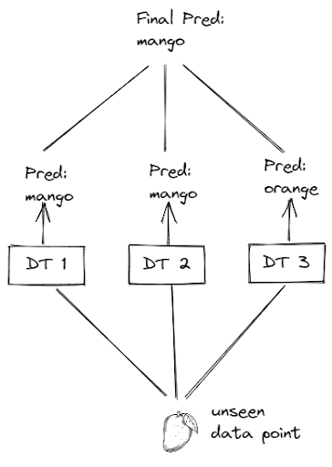
The good thing about the Random Forest algorithm is that it aggregates the predictions of each Decision Tree model on an unseen data point, which then makes the prediction more robust and less sensitive to small changes to our data. As you can see from the visualization above as an example, out of our three Decision Tree models, two of them predicted that our unseen data point is a mango, while the other one predicted it as an orange. However, since we aggregate the predictions of these three Decision Tree models, then we still get the right prediction in the end.
Random Forest Code Implementation
Now that we know how the Random Forest algorithm works let’s implement it in code. Same as before, we’re going to use the scikit-learn library to build the model and then train it on our original data.
import pandas as pd

shape = ['round', 'oval', 'round', 'round', 'oval', 'round', 'round', 'oval', 'oval', 'oval']
colour = ['orange', 'green', 'green', 'orange', 'green', 'green', 'green', 'green', 'orange', 'orange']
taste= ['sweet', 'sweet', 'sweet', 'sour','sweet', 'sweet', 'sour', 'sour', 'sweet', 'sweet']

label = ['orange','mango','orange', 'orange','mango', 'orange', 'mango', 'mango', 'mango', 'orange']

data = {'shapes': shape, 'colour': colour, 'taste': taste}
df_features = pd.DataFrame(data=data)
Next, let’s transform our features such that we have numerical features instead of strings
shape = pd.DataFrame(df_features.shapes.replace(['round','oval'],[0,1]))
colour = pd.DataFrame(df_features.colour.replace(['orange','green'],[0,1]))
taste = pd.DataFrame(df_features.taste.replace(['sour','sweet'],[0,1]))
df_features = pd.concat([shape, colour, taste], axis=1)
Building and training of a Random Forest model can be easily implemented with the scikit-learn library, as we only need few lines of code to do so, as you can see below:
from sklearn.ensemble import RandomForestClassifier

rf = RandomForestClassifier(random_state=2)
rf.fit(df_features, label)
And that’s all you need to do. The trained model is now ready to be used to predict the test data.
Conclusion
In this article, we have learned in-depth about the learning process of the Decision Tree algorithm, which can be used both in classification and regression tasks. Although it usually performs really well on its own, a Decision Tree algorithm itself is very prone to small changes in our dataset.
To alleviate this problem, a Random Forest algorithm provides a more robust solution by training several Decision Tree models on a different subset of data and then aggregates the prediction in the end.
Latest Posts:


Share